Stefan-Boltzmann Revisited

Limits to Growth with Physics

May 29, 2024 · John Peach

This article examines fundamental physical limits to economic growth by analyzing Earth’s energy balance using the Stefan-Boltzmann Law. Three key findings are:

Current global energy consumption (178,889 TWh/year) contributes to Earth’s temperature directly through waste heat, representing approximately 4% of Earth’s total energy imbalance.
Using a single-layer atmospheric model, we can show that each additional watt per square meter of forcing leads to roughly 0.3°K of warming, though this likely understates actual climate sensitivity due to feedback mechanisms.
Most importantly, continuing our current 2.3% annual economic growth rate (assuming direct energy correlation) would lead to catastrophic temperature increases within centuries due to exponential waste heat accumulation, regardless of energy source.

The analysis demonstrates that infinite economic growth is physically impossible on a finite planet, even with perfectly “clean” energy sources, due to fundamental thermodynamic constraints.

In our earlier article, Economics and the Stefan Boltzmann Law we showed that economic growth is limited by energy consumption because all energy rapidly becomes waste heat which must be radiated away from the Earth. Assuming an unlimited energy supply, the waste heat quickly increases until the Earth becomes uninhabitable. In reality, no energy sources exist that would allow this to happen, but it provides an absolute upper bound on growth.

An assumption is that economic growth depends on energy. Tim Garrett who is a climate scientist at the University of Utah wrote two papers on energy and economic growth, Long-run evolution of the global economy: 1. Physical basis and Long-run evolution of the global economy– Part 2: Hindcasts of innovation and growth where he estimates that to maintain $1000 of economic wealth requires 7.1 watts of constant power. Economic growth requires a surplus of energy above this minimum maintenance level.

In an interview with Rachel Donald on Planet Critical, Garrett discusses the thermodynamic relationship between energy, material consumption, and economics, in The Thermodynamics of Degrowth.

To understand the physics of energy and the Stefan-Boltzmann Law we’ll turn to another source - Limits to economic growth by Tom Murphy a professor (emeritus) in the departments of Physics and Astronomy & Astrophysics at the University of California, San Diego. From this, we’ll be able to calculate

The average Earth temperature based on incoming solar radiation
The temperature increase from radiating away heat caused by industrial activities
The temperature rise assuming constant economic growth over several centuries

The calculations will be done in a JupyterLab notebook in Julia where you can adjust parameters to see the effects. Another resource is $CO_2 \; v. \; CH_4$ where we used an SMath Studio notebook to build a single layer model of the atmosphere.

Earth average temperature

The Stefan-Boltzmann Law is

J = \sigma T^4

where

$J=$ radiant emittance in units of $\frac{W}{m^2}$
$σ=5.67×10−8 \; \frac{W}{m^2⋅T^4}$ is the Stefan-Boltzmann constant
$T=$ temperature of the blackbody radiator in degrees Kelvin

The equation is more fully explained in Murphy’s free online textbook, Energy and Human Ambitions on a Finite Planet in §1.3 Thermodynamic Consequences. The Stefan-Boltzmann Law relates the power $P$ radiated from a blackbody, or perfect radiator, with surface area $A_{surf}$ to the temperature of the body $T_{hot}$ radiating into a background at temperature $T_{cold}$ .

P=A_{surf} \sigma (T_{hot}^4−T_{cold}^4)

The Earth radiates into space with a background temperature so cold that it can effectively be set to zero, reducing the equation to $P = A_{surf} \sigma T^4$ .

The radius of the Earth is $R_{\oplus} \approx 6.371e6 \; m$ and the power of the sun is about $F_{\odot} = 1360 \frac{W}{m^2}$ at the top of the atmosphere. All light from the Sun that reaches the Earth passes through a disk with area $A_{disk} = \pi R_{\oplus}^2$ and is radiated into space from the full surface of the Earth with area $A_{surf} = 4 \pi R_{\oplus}^2$ . Not all of the energy reaches the surface, so a correction term needs to be included to account for the albedo, $\alpha \approx 0.293$ . Thus,

P_{in} = F_\odot (1 - \alpha) \pi R_\oplus^2 = 960 \pi R_\oplus^2

and

P_{out} = 4 \pi R_\oplus^2 \sigma T^4.

Solving for $T$ ,

T = \left( \frac{960}{4 \sigma} \right)^{1/4}

giving an average temperature, $T = 255 \degree K$ . This is about $\Delta T_{GHG} = 33 \degree K$ colder than the observed average temperature because greenhouse gases in the atmosphere trap some of the escaping energy giving a mean surface temperature, $T_{Earth} = T + \Delta T_{GHG} = 288 \degree K \;(14.85 \degree C, 58.73 \degree F)$ .

Temperature increases from energy use

Almost all energy is quickly converted to heat which must be radiated away as infrared energy to maintain the Earth’s energy balance. Exceptions to this are emissions in other wavebands directly into space such as radio waves or light. Compared to the energy used by heat-producing equipment, these sources are relatively small.

Total energy consumption worldwide in 2022 was $E = 179819 \; \text{TWh}$ (1 terawatt $= 1 \times 10^{12}$ watts) per year. To convert this to power, divide by the number of hours in a year because energy is power times time. Let $H = 365 \text{ days} \times 24 \frac{\text{hours}}{\text{day}} = 8760 \text{ hours}$ . The constant power consumed is

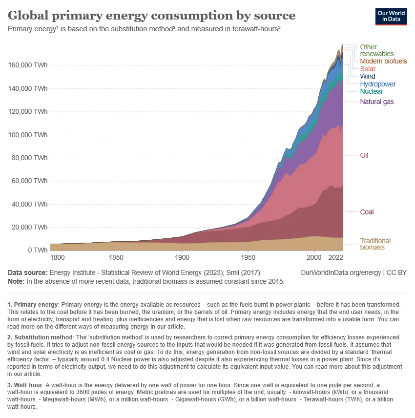
P_0 = \frac{E}{H} = \frac{179819 \text{ TWh}}{8760 \text{ hours}} = 20.52e12 \text{ watts}.

global-energy-substitution — Figure 1.
Global primary energy consumption.

For convenience, if we divide $P_0$ by the area of the Earth’s disk, then this power can be combined with the solar input $P_{in}$ as if it were evenly distributed over the same area. Since $A_{disk} = \pi R_\oplus^2 = 1.275e14$ then the power per square meter is

p_0 = \frac{P_0}{A_{disk}} = \frac{P_0}{\pi R_\oplus^2} = \frac{179819}{1.275e14}.

The combined power from the Sun and energy consumption per square meter over the Earth’s disk is

p_{in} = F_\odot (1 - \alpha) + p_0

and the power radiated out per square meter is $p_{out} = 4 \sigma T^4$ . Equating $p_{in} = p_{out}$ and solving for $T$ ,

\begin{aligned} \Delta T_{Energy} &= \left( \frac{F_\odot (1 - \alpha) + p_0}{4 \sigma} \right)^{1/4} + \Delta T_{GHG} - (T + \Delta T_{GHG})\\ &= \left( \frac{F_\odot (1 - \alpha) + p_0}{4 \sigma} \right)^{1/4} - T = 0.0106 \degree K. \end{aligned}

In Julia, this can be written as a function:

TE(E) = map(e -> ((F*(1-α)+e/(H*A_disk))/(4*σ))^0.25 + T_GHG, E)

which gives TE(E) - TE(0) = 0.010624. According to the paper Observational Assessment of Changes in Earth’s Energy Imbalance Since 2000 by Loeb et al, the Earth’s Energy Imbalance is now $1.0 \pm 0.2 \frac{W}{m^2}$ . In Recent reductions in aerosol emissions have increased Earth’s energy imbalance the authors find that reductions in aerosol emissions are causing an acceleration of the imbalance.

Letting

EEI = 1.0 \frac{W}{m^2} \cdot H \frac{hrs}{year} \cdot A_{surf} \; m^2 = 4.47e6 \; TWh

From the function TE,

TE(EEI) - TE(0) = 0.265

while

TE(E) - TE(0) = 0.0106

which means that about 4% of the total energy imbalance is due to direct heating from human activities. The ratio of the energy consumed $E$ , to the energy due to greenhouse gas imbalance $EEI$ is $E/EEI = 0.04$ , so also about 4%.

The single-layer model

In the earlier article showing how to model the term $T_{GHG}$ for temperature increase due to greenhouse gases can be more accurately approximated with a single-layer model of the atmosphere.

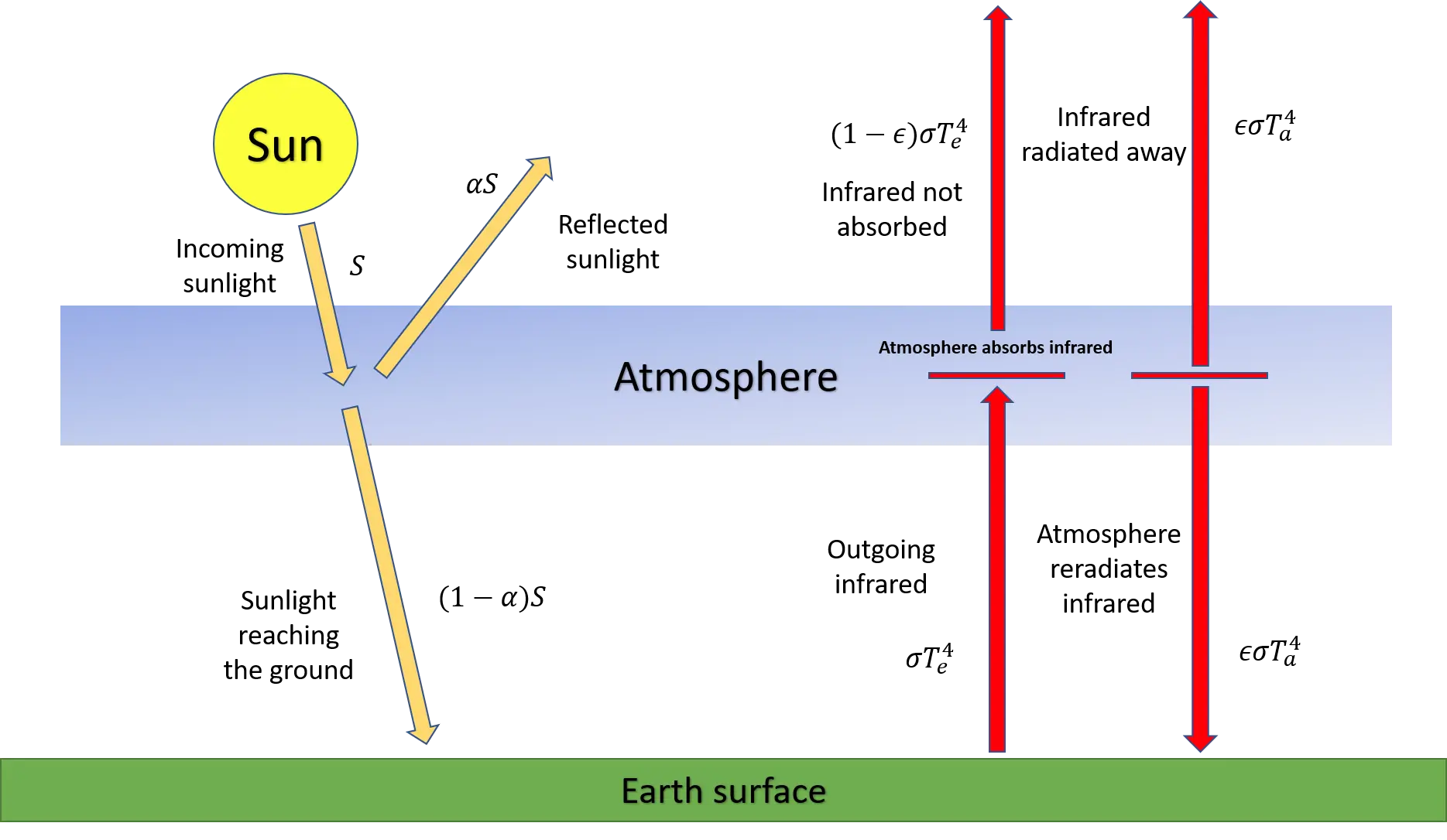
single-layer-model-complete — Figure 2.
Single layer energy balance model.

The equation we used was

T_e = \left( \frac{(1-\alpha)S}{(1 - \frac{\epsilon}{2}) \sigma} \right)^{1/4}

where $S = F_\odot / (A_{surf}/A_{disk}) = F_\odot/4 = 341.25 \frac{W}{m^2}.$ We used $F_\odot = 1365$ previously. This model includes an emissivity term $\epsilon = 0.78$ to account for the transmission of energy through the atmosphere. This equation gives the temperature in terms of power per square meter of the Earth’s surface.

A simple modification lets us calculate the temperature with an additional power term, $p$

T_e(p) = \left( \frac{(1-\alpha)S + p}{(1 - \frac{\epsilon}{2}) \sigma} \right)^{1/4}.

With no additional sources, $T_e(0) = 288.73 \degree K$ as expected. Adding the forcing term from greenhouse gases of $1 \frac{W}{m^2}$ and subtracting $T_e(0)$ gives

Te(1) - Te(0) = 0.2998

The calculated temperature increase of $0.3\degree K$ for an additional $1\frac{W}{m^2}$ of forcing seems too low compared to observed climate sensitivity, which typically ranges from $0.4$ to $1.2 \degree K$ per watt of radiative forcing. Here are some reasons why:

Climate sensitivity: The equation assumes a constant climate sensitivity, which is the equilibrium temperature change resulting from a doubling of atmospheric CO2 concentration. However, in reality, climate sensitivity is not constant and can be influenced by many factors.
Climate Feedbacks: The model does not include feedback mechanisms such as changes in water vapor, ice-albedo feedback, cloud cover changes, and others, which can amplify the warming effect.
Simplifications: The equation assumes a simple balance of incoming and outgoing radiation without considering the complex energy exchanges within the Earth’s climate system.
Radiative Forcing Efficacy: Different greenhouse gases have different efficacies in terms of how much they contribute to radiative forcing per unit increase in concentration.
Non-gray atmosphere: The assumption of a gray body atmosphere, where the atmosphere has a constant emissivity and absorptivity independent of wavelength, is an oversimplification. The Earth’s atmosphere has a more complex spectral behavior, with greenhouse gases absorbing and emitting differently at different wavelengths.

The simplified model gives a basic estimate but lacks the complexity required to match observed temperature increases accurately. Real-world climate sensitivity is influenced by a variety of feedback mechanisms and interactions not captured here. While useful for a basic understanding, more comprehensive climate models are needed for accurate predictions.

The Stefan-Boltzmann Law is well established in physics, but the Earth’s climate system is much more complex than can be captured in a simple equation. It only accounts for about 30% of the observed warming, and even if greenhouse gas emissions ended now, we might expect several decades of continued warming before the system reaches equilibrium.

Recognizing that the predicted temperature increase is lower than observations, let’s calculate the temperature under continuous economic growth, assuming that the economy is directly dependent on energy inputs.

Exponential growth

In his paper, Limits to economic growth Tom Murphy shows the exponential growth of energy consumption.

constant-power — Figure 3.
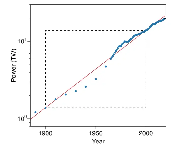
Historical energy growth.

The red line is a fit through the data points at 1900 and 2000 with annual economic growth of 2.3%. This rate of growth corresponds to a multiplier of 10 per century and appears as a straight line because the Power axis is logarithmic.

Continuing the plot for another thousand years, we can calculate the average power $q$ using

q(T) = q_0 e^{r (t - t_0)}

starting in year $t_0 = 2000$ with initial power $q_0 = 122857 \; TWh$ . Plug the output of $q(T)$ into the function $T_e$ to see the temperature of the Earth rising exponentially.

earth-temperature — Figure 4.
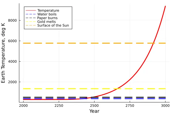
Earth temperature with continuous 2.3% annual economic growth.

So we have a choice. Do you want growth that leads to the Earth burning up in a huge ball of flame, or do you want a crashing economy?

C’mon, c’mon - it’s either one or the other.

Code for this article

The calculations were done in a JupyterLab notebook using Julia, The Stefan-Boltzmann Law Revisited. To generate the plot, install Plots.jl using the Julia package manager. To export the figure use

savefig(raw"<file directory>\earth-temperature.png")

Software

Julia - The Julia Project as a whole is about bringing usable, scalable technical computing to a greater audience: allowing scientists and researchers to use computation more rapidly and effectively; letting businesses do harder and more interesting analyses more easily and cheaply.
JupyterLab - JupyterLab is the latest web-based interactive development environment for notebooks, code, and data.
SMath Studio - Tiny, powerful, free mathematical program with WYSIWYG editor and complete units of measurements support.

References and further reading

Long-run evolution of the global economy: 1. Physical basis, Tim Garrett.
Long-run evolution of the global economy– Part 2: Hindcasts of innovation and growth, Tim Garrett.
Limits to economic growth, Tom Murphy.
Energy and Human Ambitions on a Finite Planet, Tom Murphy.
Energy Transitions: Global and National Perspectives, Vaclav Smil.
Observational Assessment of Changes in Earth’s Energy Imbalance Since 2000, Loeb et al.
Recent reductions in aerosol emissions have increased Earth’s energy imbalance, Hodnebrog et al.
Navigating Climate Catastrophe: Part 1 – The Predicament, Richard Heinberg, Resilience
Simple Earth Climate Model: Single-Layer Imperfect Greenhouse Atmosphere, Physics Teaching for the 21st Century, UBC Physics & Astronomy Outreach.

Image credits

Hero: Dealing with the Devil, Gary Larson. The 10 Best Far Side Comics, Screen Rant.
Global primary energy consumption by source, Our World in Data.
The Single Layer Model, CO2 v. CH4, Wild Peaches.
Historical energy growth: Limits to economic growth, Tom Murphy.
Earth Temperature, The Stefan-Boltzmann Law Revisited, generated in Julia.