

Hubbert Linearization
An Esoteric Concept with Extraordinary Consequences
Ask NotebookLMA prescient insight by M. King Hubbert in 1956 revealed that U.S. oil production would soon reach a maximum never to be achieved again. We’ll show the mathematics of how his method works, but also why the underlying hypothesis doesn’t hold for global energy production. Howard T. Odum’s Maximum Power Principle says that every species attempts to maximize consumption of natural energy resources at a rate that optimizes growth of the species. Humans have been following this principle during the Industrial Revolution, optimizing our numbers, but with dire consequences for ourselves and the environment.
Hubbert’s Prediction
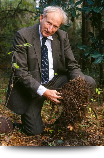
In 1956, M. King Hubbert predicted that U.S. oil production would reach a maximum sometime between 1965 and 1970, and would decline forever afterward. Hubbert was a geologist and geophysicist working for Shell Oil at the time, but he also taught at Columbia, UC Berkeley, and Stanford.
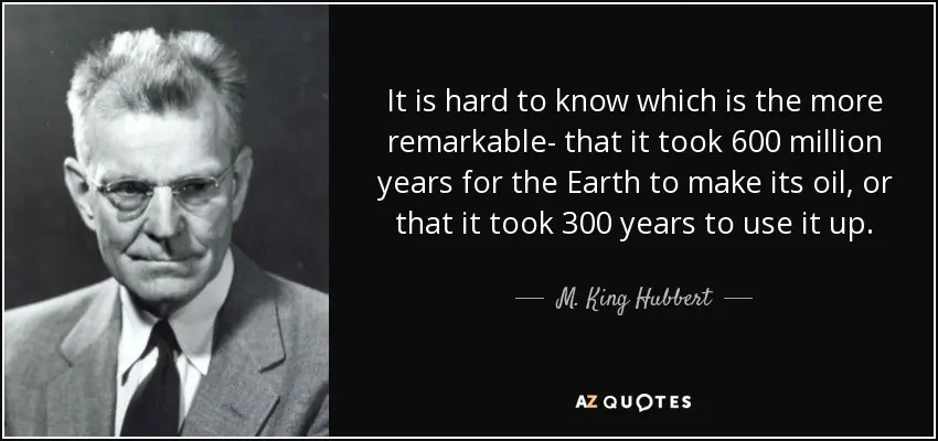
M. King Hubbert.
In fact, U.S. oil production did peak in 1970, and declined until the early 2000s when the fracking revolution began and oil production surged. How did Hubbert correctly predict the peak of production? He assumed that for any oil field there would be a time when the first few wells were drilled and oil production would be low, followed by a “gold rush” of wells extracting ever increasing quantities, and then geology constraints would lead to a slow decline.
The point of maximum production is now known as “Hubbert’s Peak” or “Peak Oil”. Hubbert modeled the production curve as the derivative of a logistic function. This meant that the cumulative production over time fitted the S-shaped curve of the logistic.
The Logistic Function
The logistic function can be expressed in several ways, but we’ll start with this:
where is the maximum height of the function, controls the steepness, and is the midpoint. In terms of non-renewable resources, the variable in the numerator represents the Ultimate Recoverable Resource (often written as ), or the total oil extracted from a field over its lifetime.
The production curve is the amount of oil produced in any year, and can be expressed as the derivative of ,
and turns out to be a function of itself. When production begins, is small and the fraction , so . Towards the end of the life of the field, , so the term on the right approaches zero and production ends.
What Hubbert realized was that by plotting against the result is a straight line. That is, divide annual production by cumulative production, and plot that on the axis with cumulative production on the axis. Notice that
The straight line is known as “Hubbert linearization”.
You can experiment with Hubbert linearization using the online scientific calculator, Desmos. Define the constants and , and then enter the cumulative and yearly production functions and . To plot the linearization, you need to define the function parametrically as a function of , so that and .
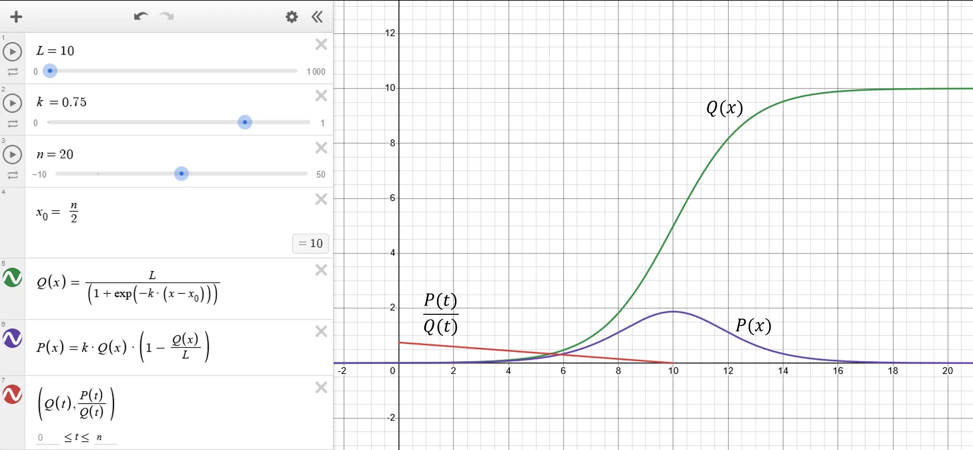
Logistic function in Desmos.
The variable is a convenience to represent the total lifespan of the field (in years). Since the peak occurs at the midpoint, we can use . Desmos creates sliders for each variable, and you can adjust the endpoints for each. The variable represents the maximum slope of , and to make the graph show actual production, set (see Appendix B. Necessary Conditions).
The convenience of Hubbert linearization is that the red line ends at , so even if the field hasn’t been fully depleted you can follow the line to the intercept with the axis and get a good estimate of how much oil the field will eventually produce.
Hubbert Linearization Applied to Energy Data
A source for energy data is Our World in Data (OWiD) founded by Max Roser in 2011, and now owned and maintained by the Global Change Data Lab.
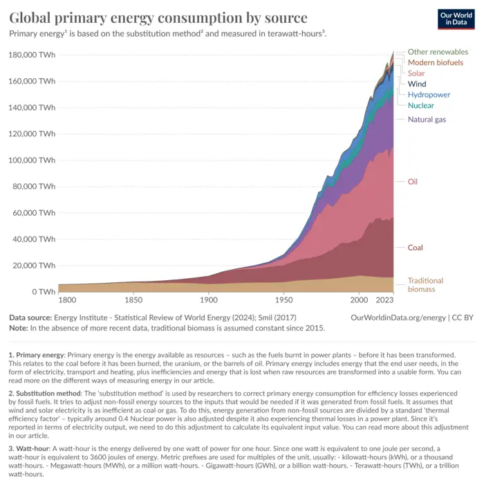
There are several serious flaws with this data. First, they use the ‘substitution method’ to attempt to make sources equal. For thermal systems that burn fossil fuels, the input fuel must be converted to heat but most of the heat is wasted. For example, a coal plant converts only 32% of the input energy contained in coal into useful electrical energy, so the OWiD multiplies the input quantity of coal by 0.32 to get the electrical energy delivered by the plant.
Wind and solar produce electricity directly, so the conversion factor is one. The problem is that fossil fuel plants can generate power to meet demand, but renewables can’t, so energy storage is required, and losses in these storage systems have not been included.
Second, there’s an implicit assumption that we can “electrify everything”. Long-haul flights, trans-oceanic tankers and freighters, and interstate trucking all require fossil fuels with no feasible alternatives currently available. The data shown here is for total global energy use, but only 20% of our current consumption is for electricity.
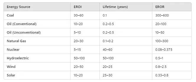
Finally, the Energy Rate of Return (EROR) is critical in understanding whether an energy system is self-sustaining. Every system requires some energy input to generate output energy. The ratio of output energy to input energy is called EROI (Energy Return over Input) and depends on energy costs to obtain, transform, and distribute the energy to the end user.
EROI is important, but it doesn’t include an estimate of how fast the initial input energy is returned. We don’t yet know what the EROR is for sustainability, but fossil fuels are obviously self-sustaining, while non-fossil systems have not been shown to be capable of rebuilding new systems using only the energy derived from a similar system. See our previous article, Burning Man for details.
EROR Estimates
Even with those caveats, though, the OWiD energy data can be useful for exploring the Hubbert hypothesis. Download the data and open it in a spreadsheet such as LibreOffice Calc. I created three new columns labeled , , and . Next, I copied one of the energy data columns into , created the cumulative sum in , and calculated in the third column.
The Hubbert plots can be generated directly from the last two columns. For non-fossil fuel sources, the plots look like this:
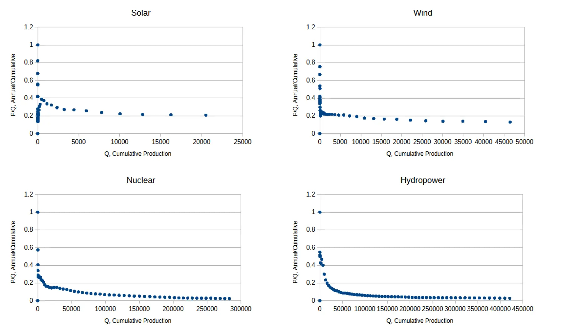
Hubbert linearization for renewables.
Looking at the general trends of these plots, we see a steady decline as annual production remains nearly constant while cumulative grows steadily, giving a linear downward slope to . If you were to plot the production to cumulative production energy for a single hydropower plant, you might expect that for the first four years of operation.
There might be minor variations in from one year to the next, but in general, it would be a relatively steady output, producing the plot shown here. New dams and power plants would modify the curve somewhat as they came online, but the overall trend would continue.
Fossil fuels should have a very different picture since the available quantities are finite, yet they also follow the same overall shape. One explanation is that there are such large quantities of remaining fossil fuels that we haven’t reached the consumption levels needed to begin seeing the linearity of Hubbert’s model.
Total world consumption of coal is estimated to be about 1.5 trillion metric tons, and remaining reserves are about 1.07 trillion metric tons, so consumption to date is about 58% of known pre-industrial revolution totals. Gas consumption is only about 22% of the total, but should be sufficient to begin seeing effects in Hubbert linearization.
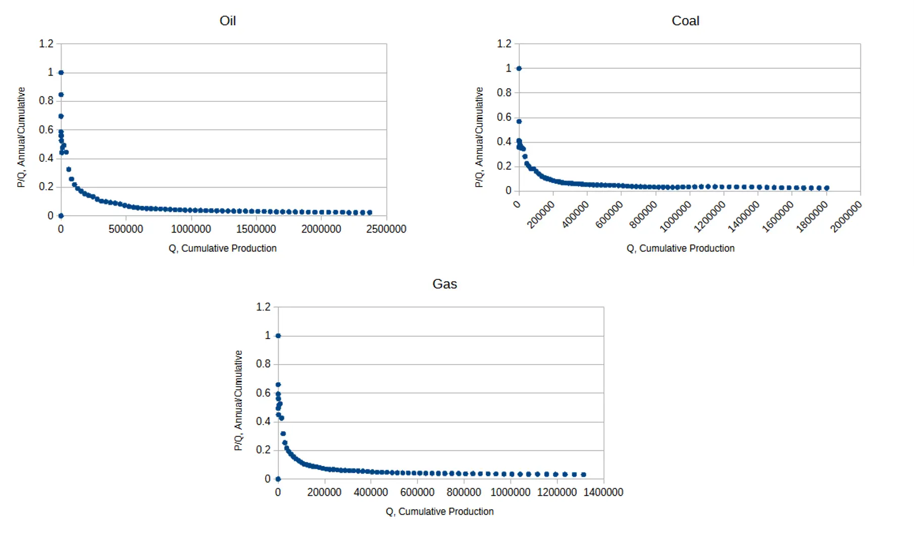
Hubbert linearization for fossil fuels.
Let’s look more carefully at the oil and coal curves, zooming in on the more recent data. Ignoring the first portion of the curve, the shape of the plot still has the same characteristic initial decline followed by a long steady descent.
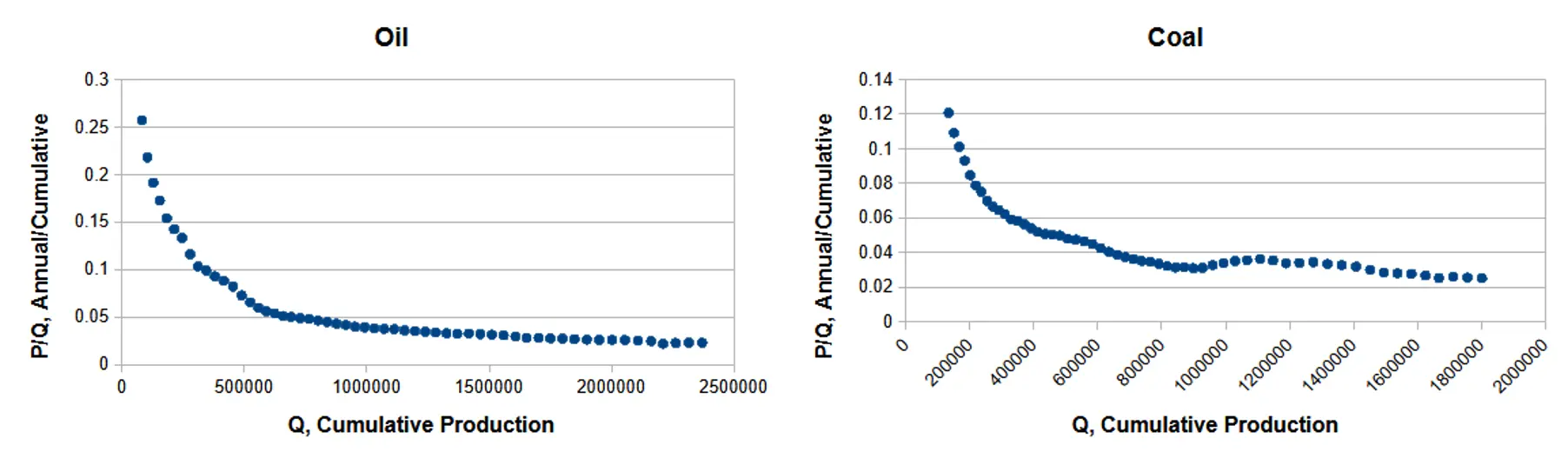
Oil and coal linearization trends showing production ratios over time.
We estimate that 2.2 trillion barrels of oil have been discovered to date, and 1.68 trillion have been produced, so consumption is about 76% of the total.
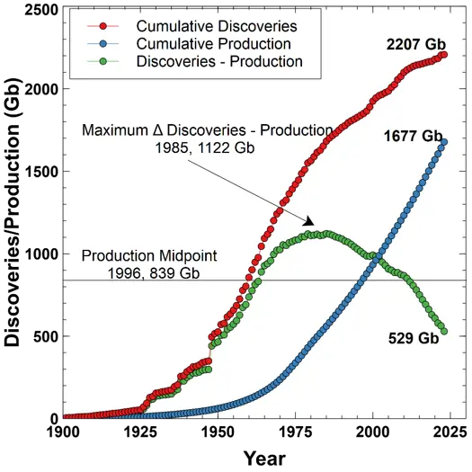
Cumulative oil discoveries and production over time.
Looking at the cumulative consumption plots from OWiD data we see that there is no characteristic S-shape to the curves. If the Hubbert principle held for world consumption of non-renewable resources, we should be seeing the effects in the cumulative consumption plots. It seems that the reason Hubbert’s model doesn’t apply to world data is a result of the Maximum Power Principle.
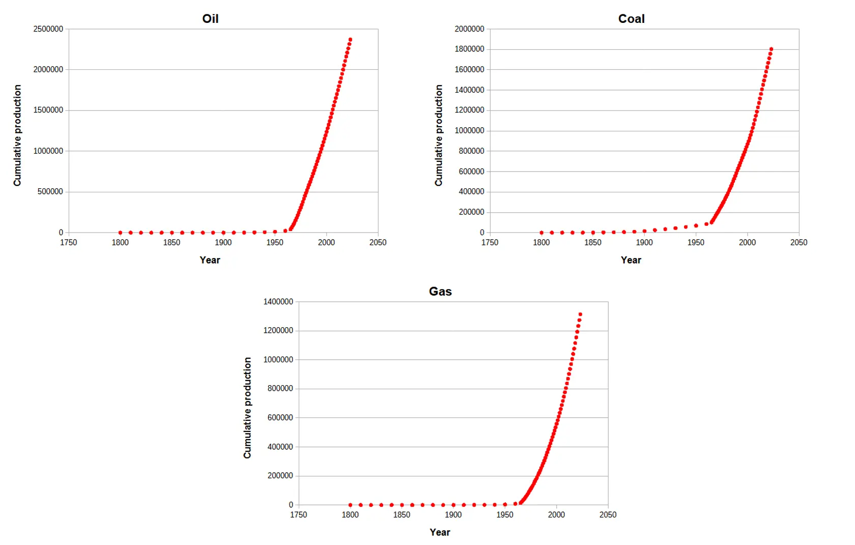
Fossil Fuel Cumulative Production.
The Maximum Power Principle
Odum’s Maximum Power Principle is a fundamental concept in systems ecology developed by Howard T. Odum in the 1950s and has implications for understanding both natural and human-made systems. Odum was an ecologist who taught at the University of North Carolina at Chapel Hill and the University of Florida.
One of his interests was systems ecology which applies systems theory, the approach to the study of ecology of organisms using the techniques and philosophy of systems analysis: that is, the methods and tools developed, largely in engineering, for studying, characterizing and making predictions about complex entities, that is, systems, as defined by ecologist Roger Kitching.
Howard T. Odum
At its core, the Maximum Power Principle states that systems that survive in competition with other systems develop designs that maximize their use of available energy. It’s not about using the least energy possible, but rather about capturing and using energy in the most effective way to ensure survival and growth.
A forest ecosystem provides a good example for understanding Odum’s idea. Trees don’t simply try to minimize their energy use. Instead, they develop complex structures - tall trunks, broad canopies, and extensive root systems - that allow them to capture the maximum amount of available solar energy and convert it into useful forms (biomass, seeds, etc.). While this might seem inefficient from a pure energy conservation standpoint, it actually represents the most successful strategy for long-term survival and reproduction.
In human systems, the Maximum Power Principle applies to everything from economic markets to cities. For instance, successful cities tend to develop infrastructure and networks that maximize their ability to process and utilize available resources, whether those are physical resources like food and water or more abstract resources like information and human capital.
What makes Odum’s principle particularly valuable is how it connects to other fundamental concepts in thermodynamics and evolution. It builds on the Second Law of Thermodynamics (which deals with entropy) but adds a crucial insight: systems don’t just dissipate energy randomly; they tend to organize themselves in ways that maximize their energy-processing capabilities.
One way to think about this is through the analogy of a river system. A river doesn’t simply take the shortest path to the sea. Instead, it develops complex networks of tributaries and meanders that might seem inefficient at first glance. However, this apparently “wasteful” structure actually allows the river system to process more energy and material over time, creating stable, resilient patterns that can persist for millions of years.
An important nuance to understand is that “maximum power” doesn’t mean “maximum energy use” - it refers to the optimal rate of energy transformation that allows a system to persist and thrive over time. Systems that process energy too quickly burn themselves out, while those that process it too slowly get outcompeted by more effective systems.
Viewing the fossil fuel plots in light of Odum’s Maximum Power Principle it becomes clear that humans are optimizing energy consumption, and we are likely to continue on current trajectories until we reach geologically imposed resource limits. It appears that the first limit to be reached will likely be oil, and since it is the backbone of modern economic systems the effects will likely be profound.
Another consequence of the Maximum Power Principle is that there won’t be an energy transition to renewables. Instead, we will continue increasing consumption of all forms of energy while we can. This becomes apparent in the OWiD energy chart above which shows all forms of energy use in greater use over time. We never switched from one source to another simply because one was more economical than another.
Appendix
A. The Logistic Derivative
Here we derive the equation for production in terms of cumulative production , assuming is logistic.
From
and recalling the quotient rule for derivatives,
and letting
we get
B. Necessary Conditions
What conditions are imposed on the parameters and to ensure the model is physically realistic? The value is the maximum quantity recovered so must be greater than zero and must be the maximum value of . A second constraint is that production should never exceed cumulative production , and this puts limits on the steepness coefficient .
For , both and is monotonically increasing, . Since is the integral of , what conditions on and are required for ? This represents the condition that is the cumulative production of a non-renewable resource.
From the results above,
so
Since , then and for , this implies that .
Code for this article
To reproduce the logistic function, open the Desmos Scientific Calculator in your browser and enter the variables and the equations as shown. Set limits for the variables such as , and . The upper bound on shown above is , but that will allow a very high peak for , and isn’t necessary for demonstrating the principles.
Software
- Desmos - Desmos is an advanced graphing calculator implemented as a web application and a mobile application.
References
- Nuclear Energy and the Fossil Fuels. M.K. Hubbert, Presented before the Spring Meeting of the Southern District, American Petroleum Institute, Mar 7-9, 1956.
- M. King Hubbert. Ron Schuler Oct 5, 2005.
- Logistic function. Wikipedia.
- Hubbert Math. Jon Claerbout and Francis Muir, Stanford University, 2020.
- EROEI and Civilization’s Forced Decline. Collapse 2050
- Burning Man. John Peach and Erik Michaels, Wild Peaches Oct. 23, 2024.
- A critique of Hubbert’s model for peak oil. Trevor H. Jones and N. Brad Willms, FACETS Volume 3, Number 1, October 2018.
- Howard T. Odum: History and Legacy. M.T. Brown, C.A.S. Hall, S.E. Jorgensen, et al. International Society for the Advancement of Emergy Research
Image credits
- Hero: An abstract art representation of Hubbert’s Peak for oil production. DreamStudio AI art generator.
- M. King Hubbert, AZ Quotes.
- Hubbert Linearization, Desmos Scientific Calculator.
- Global primary energy consumption by source, Our World in Data.
- Howard T. Odum: History and Legacy, International Society for the Advancement of Emergy Research.