

World Fossil Fuels Discoveries and Production
An analysis of current reserves
Ask NotebookLMAbstract
This study reassesses the size and reliability of global fossil fuel reserves by analyzing discovery, production, and backdated resource data for oil, natural gas, and coal. Using imputed field-level data from Global Energy Monitor, historical production records, and reserve benchmarks from the Energy Institute, we construct a bottom-up estimate of cumulative discoveries and remaining reserves. A generalized Richards growth model is applied to reconstructed discovery series for each fuel, enabling comparison between official proved reserves and geologically inferred ultimately recoverable resources (URR).
Results indicate that global discoveries of oil, gas, and coal all peaked between 1950 and 1970, while consumption has continued to accelerate, especially in the past 30 years. For both oil and gas, remaining reserves appear smaller than cumulative production to date, and discovery flows since 2015 have replaced only 10–20% of annual extraction. These findings support earlier work by Laherrère, Smil, Odum, and Garrett, and suggest that fossil fuel availability may constrain future economic activity far earlier than is implied by official reserve statistics. The analysis underscores the need for greater transparency in reserve reporting, improved discovery datasets, and a more integrated energy–economy modeling framework to understand the implications of a resource-constrained future.
Executive Summary
The global energy system remains overwhelmingly dependent on fossil fuels, yet the geological basis for this dependence is eroding. This report re-evaluates the remaining global endowment of oil, natural gas, and coal using backdated discoveries, historical production records, and generalized Richards curve modeling. Discovery data estimated by geoscientists on-site, rather than industry reports, shows that all three fossil fuels peaked in discovery between 1950–1970.
Key findings:
- Oil, gas, and coal discovery rates have declined for 50–70 years.
- Since the early 1980s, oil and gas production has consistently exceeded discovery.
- Half of all oil consumed in human history was burned in the last ~ years.
- Oil’s geologically inferred remaining reserves is Gb (1 Gb = 1 billion barrels) — far below official estimates.
- Estimated reserves provide only 25 years of continued consumption at current rates.
- Gas shows a similar trajectory; coal is abundant in mass but constrained by grade and geography.
- Energy consumption continues rising, consistent with Odum’s Maximum Power Principle and Garrett’s thermodynamic economic model: economic growth tightly tracks energy throughput.
Fossil fuels remain essential for heavy transport, fertilizers, industrial heat, shipping, and aviation—domains where renewable electricity offers no substitute. Given the accelerating decline in field quality and discovery, society must prepare for a post-growth, resource-constrained future. While production and consumption data are relatively transparent, estimates of remaining reserves vary widely and are often proprietary, politicized, or economically constrained.
In this article, we ask: How robust are the world’s fossil fuel reserves when inferred from geological discoveries rather than reported by states or firms? Using historical production records, field-level discovery data, and imputation of missing values, we compare backdated discovery trends with officially reported proved reserves to assess the reliability of current estimates and identify possible shortfalls.
The results challenge common assumptions about energy abundance and suggest that the margin for continued growth may be far narrower than expected.
Introduction
In 1956, M. K. Hubbert, a petroleum geologist then working for Shell Oil, hypothesized that U.S. oil production would reach a maximum between 1966 and 1970, and decline afterward due to geological constraints. He based his hypothesis on the observation that individual wells tend to follow a logistic derivative model, or “bell-shaped” curve. Extrapolating this to fields, he found the same model held and he expected it to hold for countries, and for the entire world. Oil production in the United States did reach a maximum in 1970 and declined until the early 2000s when hydraulic fracturing (“fracking”) was implemented on a wide scale and new peaks of production were achieved [16].
Many have taken Hubbert’s model to be the correct method for predicting worldwide oil production because the model held for decades. Even the advent of fracking could be thought of as a bell-curve added to the existing bell-curve of conventional oil. The logistic derivative is symmetric about the maximum, leading many to believe that once a global peak arrived, it would indicate a half-way point, and geological constraints would allow a smooth descent in petroleum use.
In fact, there has been no indication in the data of energy consumption that production is following the Hubbert model. The pattern instead has been one of increasing consumption of all forms of energy over time. Ecologist Howard T. Odum developed the Maximum Power Principle which asserts that ecological systems that survive in competition with other systems develop governing principles that maximize their use of available energy. It’s not about using the least energy possible, but rather about capturing and using energy in the most effective way to ensure survival and growth.
What makes Odum’s principle particularly valuable is how it connects to other fundamental concepts in thermodynamics and evolution. It builds on the Second Law of Thermodynamics (which deals with entropy) but adds a crucial insight: systems don’t just dissipate energy randomly; they tend to organize themselves in ways that maximize their energy-processing capabilities.
Tim Garrett, a climate scientist at the University of Utah, found that it takes 7.1 watts of continuous power to maintain $1000 of wealth (in 2005 U.S. dollars). World GDP is almost perfectly correlated with energy consumption, so growth of the economy requires growth in energy consumption. The analyses by Odum and Garrett contradict Hubbert’s model of a peak in production, and they more closely align with historical consumption data.
However, discovery of fossil fuel reserves appears to be following the Hubbert model where peaks in oil, natural gas and coal occurred in the 1965-1970 era, and have generally been declining since. In this study, we examine historical records of discoveries, production and estimated reserves for the three fossil fuels currently powering modern society.
We consider three broad categories of fossil fuel data - discoveries, production and consumption, and reserves. Of these, production data may be the most reliable simply because production involves multiple financial transactions which require two parties to agree on both price and quantity. We also believe that discovery data is fairly reliable because petroleum geologists must assess the quality of the field and expected content after the play or mine has been discovered.
Fossil Fuels History
Oil
Oil (crude petroleum) formed from ancient marine microorganisms—algae and plankton—that settled to the seafloor millions of years ago. Buried under sediments, they were cooked by heat and pressure into waxy kerogen and then into liquid hydrocarbons that migrated into porous reservoir rocks capped by impermeable seals. Early “discoveries” were often natural seeps used for lighting and medicine; modern exploration relies on seismic reflection imaging, geological basin modeling, and exploratory drilling, with geosteering to stay within thin, high-quality layers.
Production typically starts with primary recovery (natural reservoir pressure and pumps), moves to secondary methods (waterflooding), and sometimes to tertiary or “EOR” Enhanced Oil Recovery techniques (CO₂ injection, thermal, chemical) to coax out remaining oil. Oil is produced onshore and offshore, from giant conventional fields to tight formations developed with horizontal drilling and hydraulic fracturing. After separation and stabilization at the field, crude goes to refineries where it is distilled and transformed into transportation fuels such as gasoline, diesel, jet fuel, and non-fuel products—petrochemical feedstocks, lubricants, solvents, and asphalt. Oil’s energy density and liquid form make it dominant in transport and crucial to plastics, fertilizers, and countless industrial supply chains.
Oil plays are classed by the expected quantities to be ultimately recovered. The quantity of oil thought to be extracted with 90% probability is listed as 1P (proved), 50% probability is called 2P (proved and probable) and 3P includes possibly economically recoverable reserves. The 1P value is necessarily the smallest to account for the highest probability of recovery, while 3P quantities are the largest. Statistically, the 2P values represent the maximum likelihood and are the values we use here [26,29].
Discovery data is often amended years after the initial discovery as data about the field improves. For example, if a play discovered in 1965 is initially assessed to have 100 Mb (million barrels) of technically recoverable oil, the value might be revised in 1970 to include another 10 Mb. This raises the question - should the 10 Mb discovered in 1970 be considered new in the year of discovery, or should it be “back-dated” to the year when the play was first found?
Jean Laherrère and other geoscientists argue that back-dating helps keep discovery data aligned with geological exploration efforts, not economic revisions or appraisal updates [16]. The oil was geologically present at the time of initial discovery, even if it wasn’t immediately recognized. Understating the true size of the discovery in early years and overstating in later years creates a false impression of sustained discovery success. Back-dating anchors resource growth to the point of geologic encounter, not human interpretation.
Counterarguments are that industry prefers “as-appraised” dates to match decision-making and investment cycles. Petroleum companies (under SEC and other rules) report reserves based on proved recoverable volumes, not ultimate geology. If the increase is due to a new zone, deeper well, or advanced seismic data, then it is a new discovery in a practical sense.
Since our concern is the geological sizes of fields rather than financial concerns, we use back-dating method to assess discoveries.
The largest field ever found is Ghawar in Saudi Arabia, discovered in 1948, but excepting that one giant field, petroleum field discoveries peaked in 1964 with the Samotlor field in Eastern Siberia. Production increased exponentially until the early 1970s, but has increased only linearly since, and with a few exceptions production has exceeded discoveries since the early 1980s. In 2024, oil production was 31.8 Gb while discoveries were only 3 Gb.
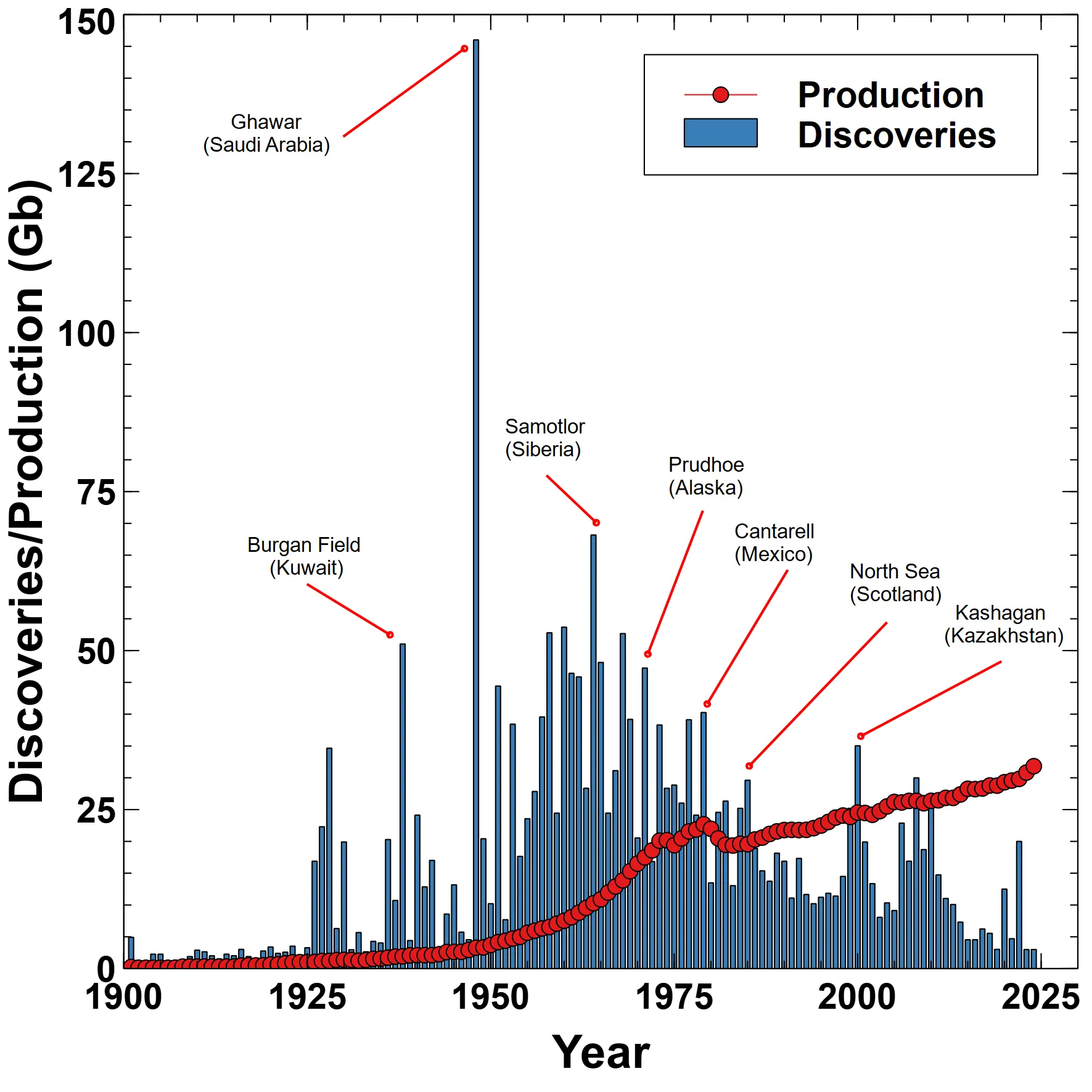
Oil discoveries and production.
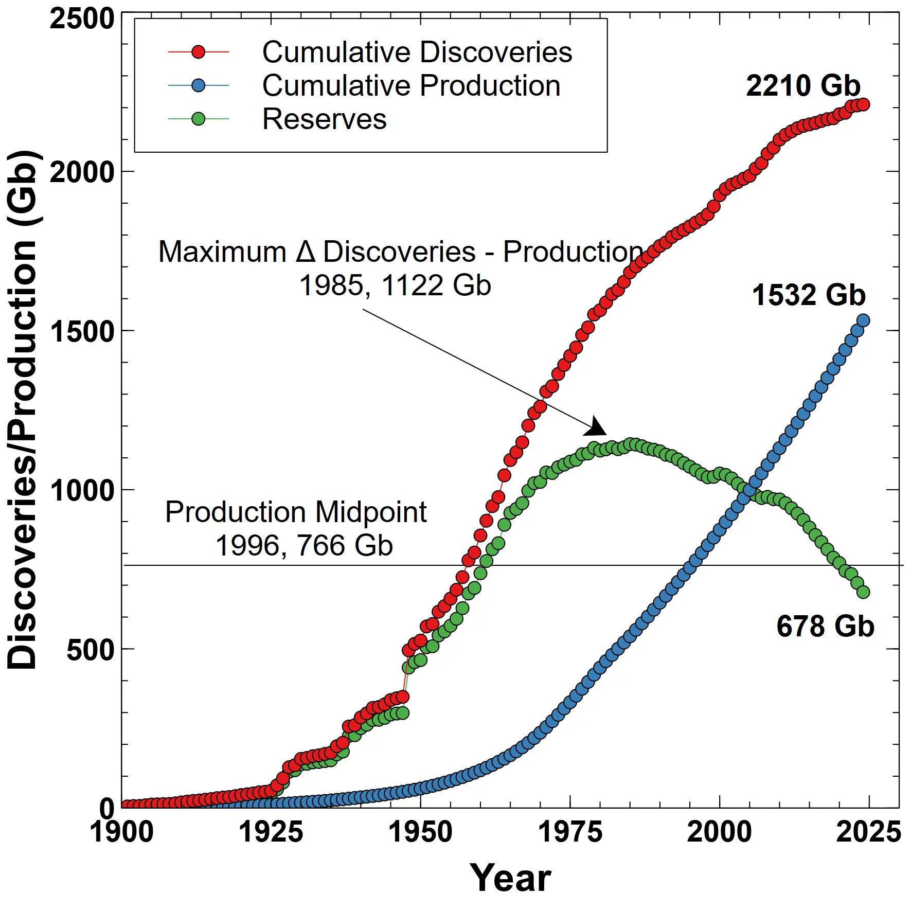
Cumulative discoveries to date have been 2210 Gb, while cumulative production of petroleum is 1531 Gb, leaving an estimated 678 Gb remaining without further discoveries [14,33]. The maximum difference occurred in 1985 at 1143 Gb, and the midpoint of total oil production worldwide was less than 30 years ago in 1996.
Oil cumulative discoveries, production and reserves.
Reserve estimates vary widely with many putting the value near 1650 Gb. The combined Canadian and Venezuelan reserves of 470 Gb exceed the Saudi Arabian estimates of 267 Gb, but this does not account for the quality of the reserves. One important measure of quality is the energy cost of extraction, transportation and refinement. Hall [40] developed the concept of “Energy Return on Investment” (EROI) which is the ratio of energy available for use to society to the energy required to process the fuel.

Estimated world oil reserves.
During the early years of petroleum use the EROI may have been as high as 100, but declined to 30 by the 1950s and is currently below 20. Oil from Saudi Arabia has the highest EROI of any source, but the tar or oil sands in Canada and Venezuela may be as low as 4:1. Without higher grade oils available to operate the machinery required to extract tar sands, it may be uneconomic to continue their extraction.
The reported reserves of OPEC countries have increased by 750 Gb since 1980 with 285 Gb from Venezuela alone. The change in Venezuelan reserves is likely due to apparently favorable extraction costs for oil sands, while other OPEC countries claimed large estimated increases in reserves during the 1980s. This has led some to question whether the reserves have been overstated as much as 300 Gb by OPEC member nations and by 100 Gb in the former Soviet Union [16]. Canadian reserves jumped from 50 Gb in 1998 to 181.5 Gb in 1999 largely due to increased estimates of tar sands economic recovery.

OPEC claimed reserves, 1980-2020.
While the true quantity of oil reserves remains unknown, policy makers should be aware of the discrepancies and unexplained increases in claimed reserves, and need to account for differences in EROI between sources.
Natural Gas
Natural gas forms alongside oil or from deeper, hotter maturation of organic matter; it can be “associated” (co-located with oil) or “non-associated” (gas-only reservoirs). Like oil, early use drew on seeps and shallow wells. Today, exploration uses the same seismic and basin tools, with attention to pressure, seal integrity, and source maturity. Gas occurs in conventional traps and in unconventional accumulations such as shale gas and coalbed methane.
Production involves drilling and completion (often horizontal in shales), followed by gathering to processing plants that remove water, CO₂, H₂S, and heavier liquids (natural gas liquids: ethane, propane, butanes). From there, gas moves by pipeline or is cooled to –162 °C to make liquified natural gas (LNG) for ship transport.
Uses include power generation via fast-ramping turbines, space and process heating, and in industry. As a chemical feedstock, methane is used to make hydrogen, ammonia and ammonia-based fertilizers and, via ethane cracking, the building blocks for plastics. Its high hydrogen-to-carbon ratio gives it lower CO₂ per unit energy than coal or oil when burned, though methane leakage management is essential given the disproportionately large global warming impact of unburned methane emissions.
Gas and oil are often associated in the same reservoir, but field data obtained from the Global Oil and Gas Extraction Tracker (GOGET) provides only the total volume in million cubic meters. Many methods have been developed to estimate the gas to oil ratio (GOR), e.g. Baniasadi et al.,
where is the solution gas-oil ratio (scf/stb) which is the volume of gas at standard temperature and pressure (scf = standard cubic foot) which will dissolve in a unit volume of oil (stb = stock tank barrel, 42 gallons) at the pressure and temperature found in the reservoir. The API is a measure of oil viscosity, is the bubble point pressure, and is the gas specific gravity, and is an empirically derived constant.
In the absence of field specific parameters, regional gas-oil ratios may be substituted [12]:
| Region / Basin | Approximate Gas Fraction | Supporting Notes |
|---|---|---|
| Middle East & MENA | ~10–20 % | Low GOR; majority oil fields |
| North Sea | ~30–40 % | Associated gas from mature oil reservoirs |
| Permian Basin (US) | ~34–40 % (recent years) | Rising gas output in shale plays |
| North America other (US/Canada) | ~30 % | Mixed proportion outside tight oil cores |
| Global average fallback | 20 % | Good fallback when no region-specific data |
There are also temporal trends - the Permian basin in Texas and New Mexico has seen associated gas rise from ~34% in 2018 to ~40% in 2024, and North Sea fields have risen from 30% pre-2000 to about 35%.
Production data was derived from data assembled by the Institute for Global Sustainability at Boston University, and reserve estimates from the Energy Institute Statistical Review of World Energy 2025. Production data covers the period 1900 - 2022, and the years 2023 and 2024 were obtained from the Statistical Review.
Discovery data from GOGET provides individual field data covering the period from a first discovery in Peru in 1869 to the present, but of the 7396 records 2466 did not list discovery years. A table of annual estimates of oil and gas production and reserve values provided by GOGET gives 42,769 records, of which 4875 have no data. The Statistical Review provides estimates of world gas reserves, but only for the period 1980 - 2020.
Given the sparsity of available data, a model was developed to fit the available data. We assumed that cumulative discoveries less cumulative production in any year represents known reserves. It is widely accepted that global gas discoveries peaked in the 1960s, so our model assumes a logistic distribution of discoveries centered between 1965 and 1970. Given these constraints, the model fits discovery and known reserve data to the production data.
Coal
Coal originates from dense accumulations of ancient plant material in swamps and peatlands. Over geologic time, burial, heat, and pressure drive off water and volatiles, concentrating carbon. The result spans ranks by maturity and energy content: lignite (lowest), sub-bituminous, bituminous, and anthracite (highest) [7,17,18]. Historically, coal seams exposed at the surface led to the first mines; systematic discovery followed with geologic mapping, coring, and geophysical surveys.
Production is either surface mining (strip/open-pit) where seams are near the surface, or underground mining (room-and-pillar, longwall) for deeper seams. Run-of-mine coal is typically washed to remove ash and sized for markets. Ash in unburned coal is a term of art to describe the original minerals and sediments that were incorporated into the peat and coal during formation. These include clay minerals, quartz silt, carbonates such as calcite or siderite, pyrite, and other inorganic materials.
Coal’s primary use is generating electricity, but it also provides high-temperature heat for cement and other industries. A special grade—metallurgical or coking coal—is essential for steelmaking in blast furnaces (to make coke, a porous, carbon-rich fuel and reductant). While simple to store and transport, coal is the most carbon-intensive fossil fuel per unit of delivered energy, so its use is increasingly shaped by emissions controls and alternatives.
There are approximately 4300 coal mines currently in operation worldwide, producing an estimated 7-8.5 billion metric tons annually [39].
| Rank | Country | 2023 Prod. (Mt) | % of Global Output (˜8,900 Mt) | Cumulative % |
|---|---|---|---|---|
| 1 | China | 4,362 | 49.00% | 49.00% |
| 2 | India | 969 | 10.90% | 59.90% |
| 3 | Indonesia | 781 | 8.80% | 68.70% |
| 4 | United States | 524 | 5.90% | 74.60% |
| 5 | Russia | 480 | 5.40% | 80.00% |
| 6 | Australia | 443 | 5.00% | 85.00% |
| 7 | South Africa | 238 | 2.70% | 87.70% |
| 8 | Kazakhstan | 118 | 1.30% | 89.00% |
| 9 | Germany | 102 | 1.10% | 90.10% |
| 10 | Poland | 89 | 1.00% | 91.10% |
| … | Other (~40+) | ~1,139 | 12.80% | 100% |
The energy content of various types of coal is estimated as:
| Coal Type | Typical GJ/metric tonne | EJ/metric tonne | Notes |
|---|---|---|---|
| Anthracite | 27.7 GJ | 2.77 × 10⁻⁸ EJ | Highest carbon content, fewest impurities. |
| Bituminous | 27.6 GJ | 2.76 × 10⁻⁸ EJ | Lower quality than anthracite, contains bitumen/asphalt. |
| Subbituminous | 18.8 GJ | 1.88 × 10⁻⁸ EJ | Primarily used in steam-electric power generation. |
| Lignite | 14.4 GJ | 1.44 × 10⁻⁸ EJ | Low heat content, high moisture. |
| Bituminous + Sub‑bituminous | (27.6 + 18.8)/2 ≈ 23.2 GJ | 2.32 × 10⁻⁸ EJ | Simple average of the two types. |
| Anthracite + Bituminous | (27.7 + 27.6)/2 ≈ 27.65 GJ | 2.77 × 10⁻⁸ EJ | Essentially same as pure bituminous/anthracite. |
| Sub‑bituminous / Lignite | (18.8 + 14.4)/2 ≈ 16.6 GJ | 1.66 × 10⁻⁸ EJ | Average of subbituminous and lignite. |
The heating value of coal depends on moisture, ash, carbon content, and regional geology, and for mixed types, e.g. anthracite + bituminous the values are the arithmetic average.
Primary energy
Primary energy is the energy in the natural or extracted form prior to transformation by any engineered conversion. Oil, coal and natural gas are examples of primary energy, while the mechanical energy derived from these sources to power transportation or the electrical energy from a power plant is secondary. Solar electrical energy from photovoltaic panels or electricity from wind turbines is still considered to be primary even though a conversion has occurred, e.g. the flow of wind through the turbine becomes electricity.
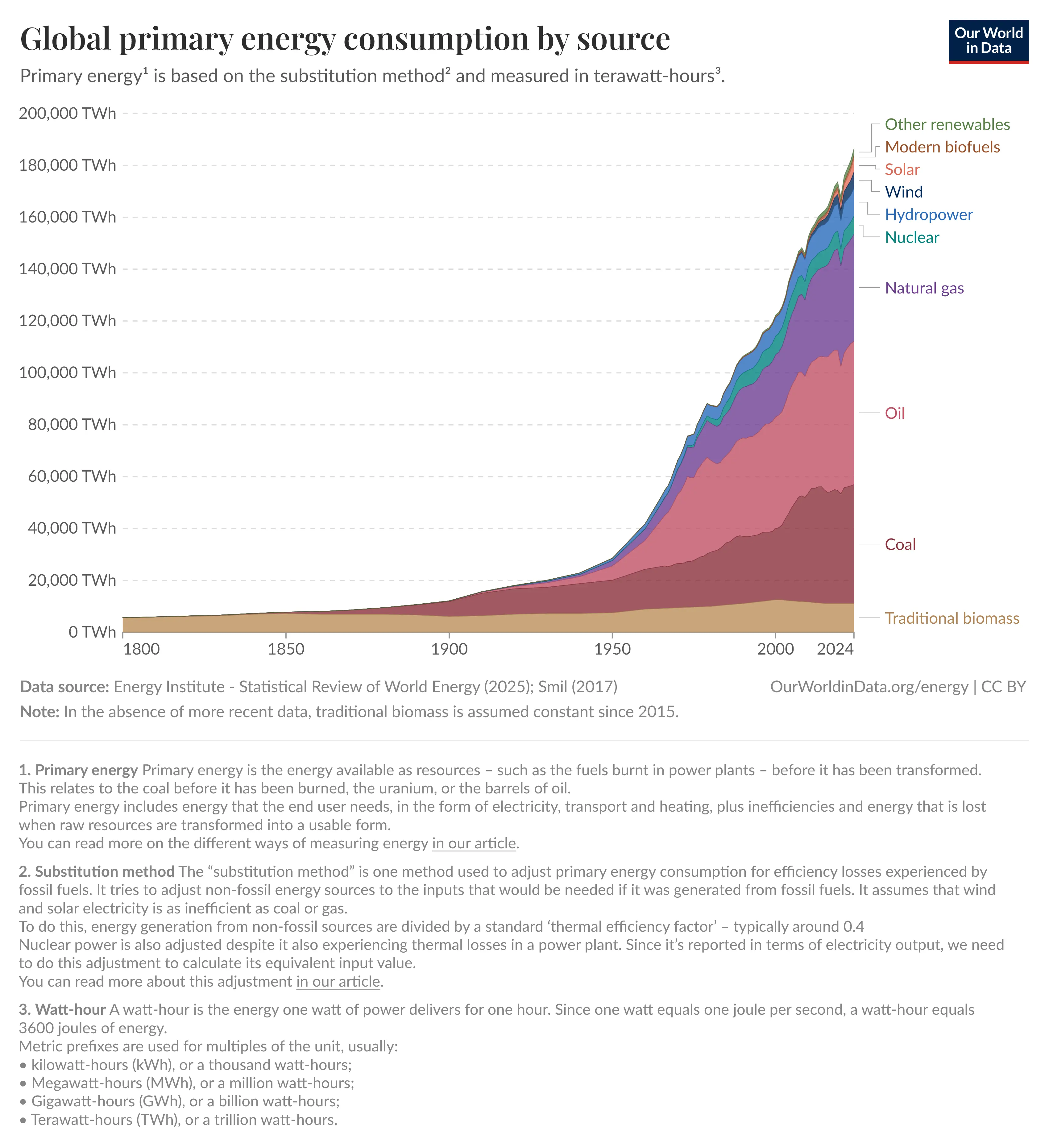
Global primary energy consumption.
Primary energy data can be quantified using two different methodologies: (1) ‘Direct’ primary energy, which directly combines fossil fuel data with the electricity generated by nuclear power and renewables. (2) ‘Substituted’ primary energy, which converts non-fossil electricity into their ‘input equivalents’: The amount of primary energy that would be needed if they had the same inefficiencies as fossil fuels. This ‘substitution method’ is adopted by the Energy Institute’s Statistical Review of World Energy, when all data is compared in exajoules.
The Substitution method attempts to create equivalencies between the primary energy sources so that they might be compared using the same TWh scale. To do this, non-fossil fuel energy sources are assumed 100% efficient in generating electricity, while fossil fuels lose 60% of source energy due to thermal inefficiencies. To correct for this, the non-fossil fuel sources are increased by 250%.
This implicitly assumes that electrical energy could power all industrial systems currently using fossil fuels. At present, there are no substitutes for petroleum derived fuels for trans-oceanic shipping, trucking and train transports, or long haul air carriers.
The second error with the substitution method is in the assumption that industrial scale electrical energy from alternative sources would be 100% efficient. Fossil fuel based power plants are able to quickly adjust loads according to demand, while none of the non-fossil sources are as resilient, with the exception of modern biofuels. In order to meet varying demand levels while adapting to supplies that fail to match the demand requirements means that energy must be stored in some form. The round-trip energy efficiency of alternate sources may not be much better than current fossil sources when storage is taken into account.
Results
The data obtained from the Global Energy Monitor Global Oil and Gas Extraction Tracker (GOGET) provides field and mine level estimates of the quantities of resources available. Small wells producing less than 1 million boe (barrels of oil equivalent) per year or have reserves of less than 25 million boe were excluded. Coal mines producing less than 1 million tonnes per annum (Mtpa) were excluded until the December 2024 update when 1,800 active coal mines with production capacities below 1 Mtpa were added to the dataset.
To estimate initial quantities in place from the GOGET data required imputation of many missing years of discovery and available resources. In addition, early year data may be incomplete. Resource quantities were backdated using the USGS modified Arrington method [19,24,25,37], and using estimated world total resource quantities for each fuel type, a Richards modified logistic was used to model historical worldwide discoveries of each resource,
with solution
where
- is cumulative discoveries at year
- represents the upper asymptote, which for resources is often called the Ultimately Recoverable Resource (URR)
- is the growth rate
- is the midpoint of discoveries, widely accepted to be in the 1960s for all three fuel types
- is the shape parameter where reduces to the standard logistic.
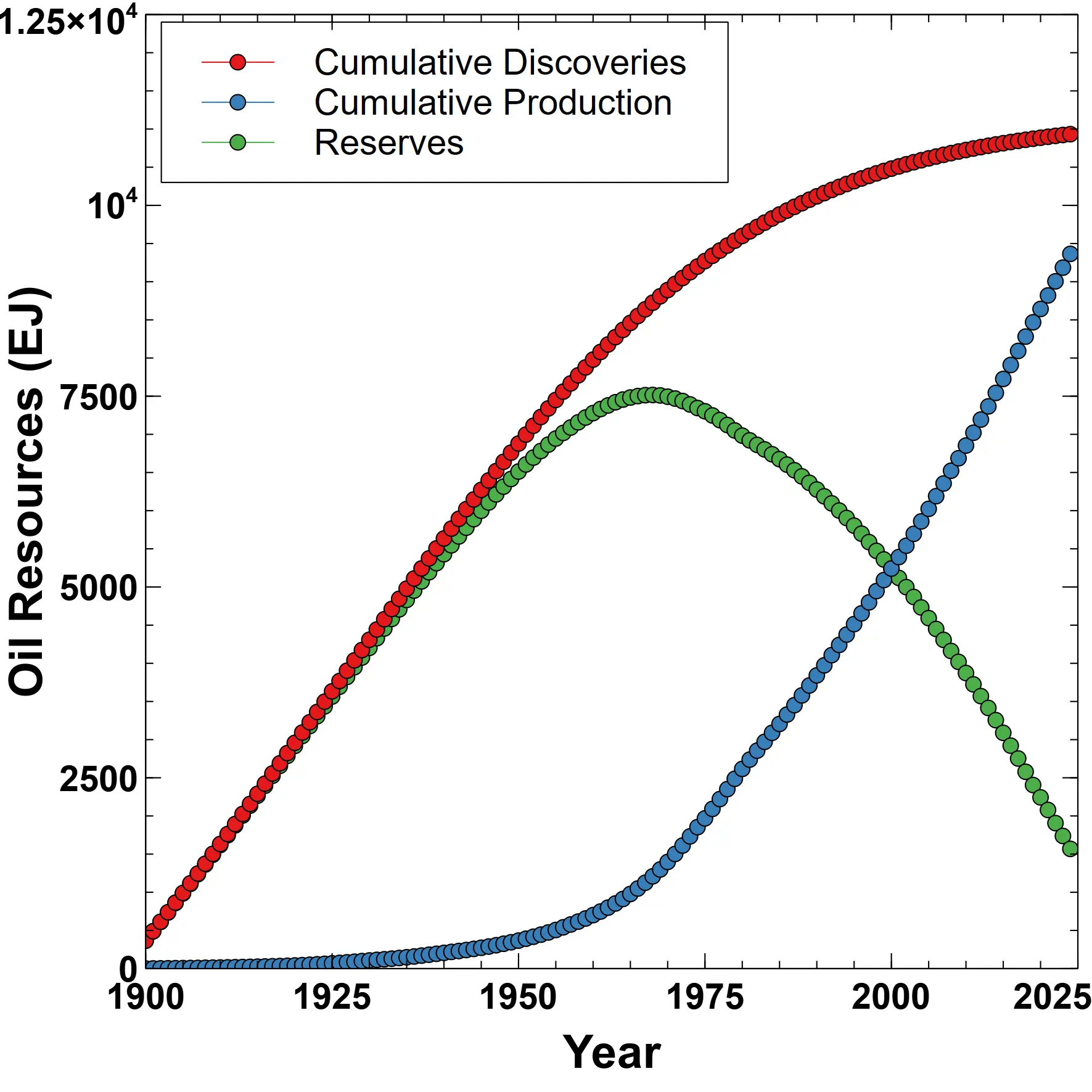
Production data was obtained from the Boston University Institute for Global Sustainability dataset, and remaining reserves are the differences between estimated cumulative annual discoveries and cumulative production. Remaining reserves as of 2020 were taken from the most recent Energy Institute Statistical Review of World Energy - 2025 report, which was used for . The Energy Institute gives world total oil reserves in 2020 as 1732.4 Gbl, which is considerably higher than our top-down estimate of 678 Gb, or the Rystad Energy estimate of 738 Gbl (2P - proven and probable) [14].
Units are in exajoules (EJ) where 1 EJ = 277.778 TWh = 1e9 KWh. This provides an estimate of remaining resources for each fuel type on a comparable scale, but is not meant to imply that fuels are entirely interchangeable. In Halfway Between Kyoto and 2050 Vaclav Smil argues that an entirely electric economy is not possible since there are no viable alternatives to heavy transport, high temperature smelting and fertilizer production [15].
Oil
GOGET oil data was fitted to the Richards model with parameters , . The sparsity of the GOGET data shows in the shapes of the curves which lack the characteristic “S” shape expected for typical resources.
Estimated oil discovery, production and reserves.
Oil production and discovery data is available from multiple sources, likely due to the outsized impact petroleum has on the world economy. Using the backdated discovery estimates of [16] shown in Figs. 1,2 an optimal fit is found by applying a Richards function (in units of Gb),

Cumulative oil discoveries Richards fit.
with an estimated Gb and peak year of 1962. may be interpreted as the maximum quantity of oil expected to be discovered, and since Gb has been produced to date, this implies a total of Gb in known and possible reserves. At current rates of Gb/year, this leaves approximately years of remaining consumption.
The fit to annual production data shows that discoveries have declined to well below current production rates. Since 2015, discoveries have been around Gb/year except in 2020 ( Gb) and 2022 ( Gb).
| Year | Discoveries | Production | Disc/Prod (%) |
|---|---|---|---|
| 2015 | 4.54 | 28.27 | 16.05 |
| 2016 | 4.54 | 28.22 | 16.08 |
| 2017 | 6.24 | 28.32 | 22.03 |
| 2018 | 5.54 | 28.79 | 19.26 |
| 2019 | 3.02 | 28.77 | 10.51 |
| 2020 | 12.50 | 29.30 | 42.66 |
| 2021 | 4.70 | 29.56 | 15.90 |
| 2022 | 20.00 | 29.82 | 67.06 |
| 2023 | 3.00 | 30.82 | 9.73 |
| 2024 | 3.00 | 31.82 | 9.43 |
Table: Oil discoveries and production since 2015 (Gb).

Annual oil discoveries Richards fit.
The Richards function assumes that during the early history of any resource, initial discovery rates are low due to low adoption rates and immature extraction technology. In the mid- century, petroleum found uses in all forms of transportation as well as other industries resulting in a discovery boom, but by the end of the century geological constraints began to impact discoveries.
The goodness of fit tests show , and a corrected Akaike Akaike is a measure of model complexity,
where is the number of fitted parameters, is the number of data points and is the residual sum of squares. While the AICc generally penalizes fits with more parameters, we fit bimodal (2 peaks) and trimodal (3 peaks) to the data and found a decrease in the AICc score. Nevertheless, we felt for simplicity to show results only for the single peak fit which gave excellent agreement with cumulative data.
Natural Gas
For natural gas, the Richards parameters were ,
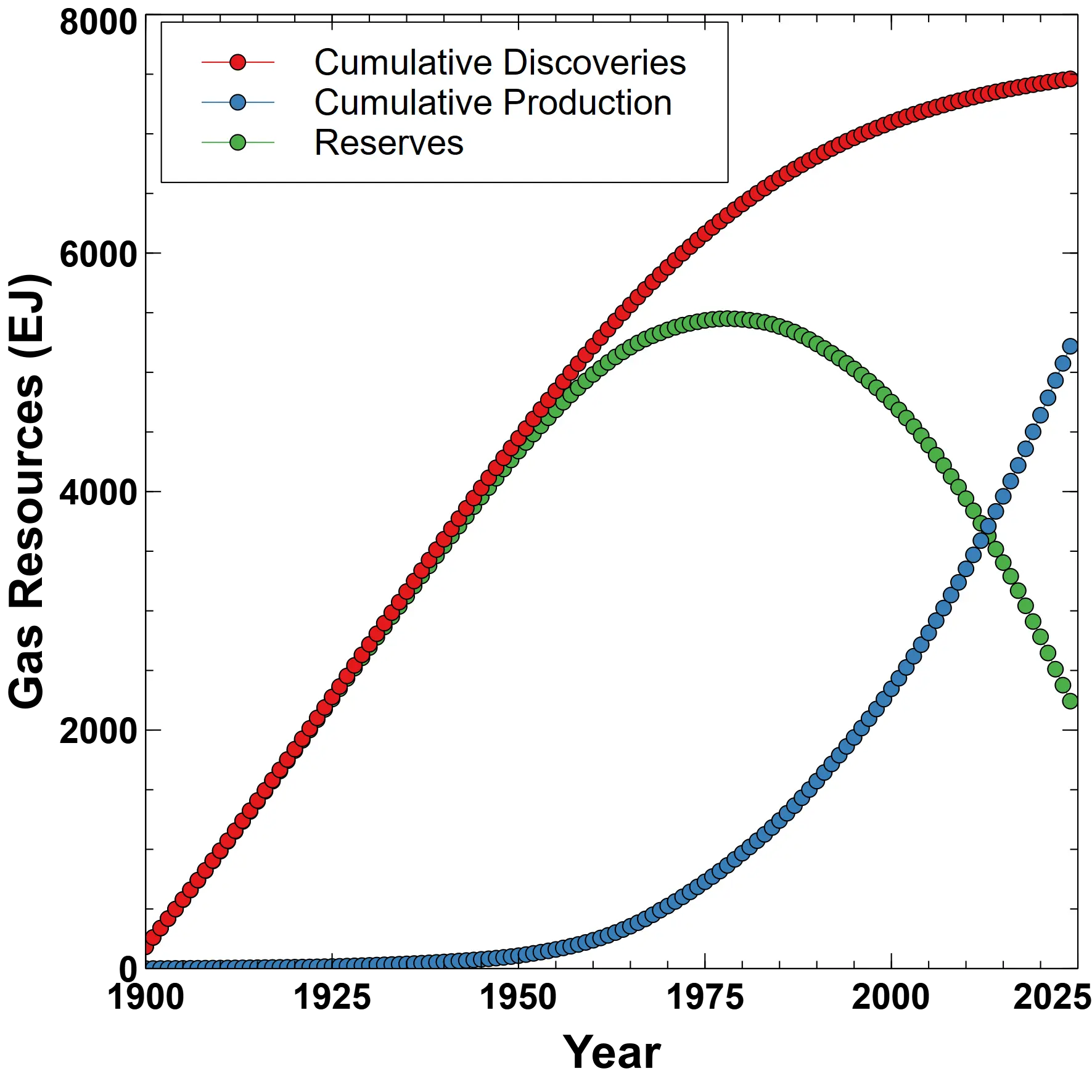
Estimated gas discovery, production and reserves.
Natural gas production (in trillion cubic meters - tcm) follows a generally upward trend and exceeds discoveries in most years after 2000. Half of all natural gas production has occurred in the last 20 years, and total cumulative production is approaching the level of remaining reserves. While it is interesting to estimate the reserve to production ratio, it should also be noted that production is generally increasing with time [31].
Coal
For coal the best fitting parameters were .
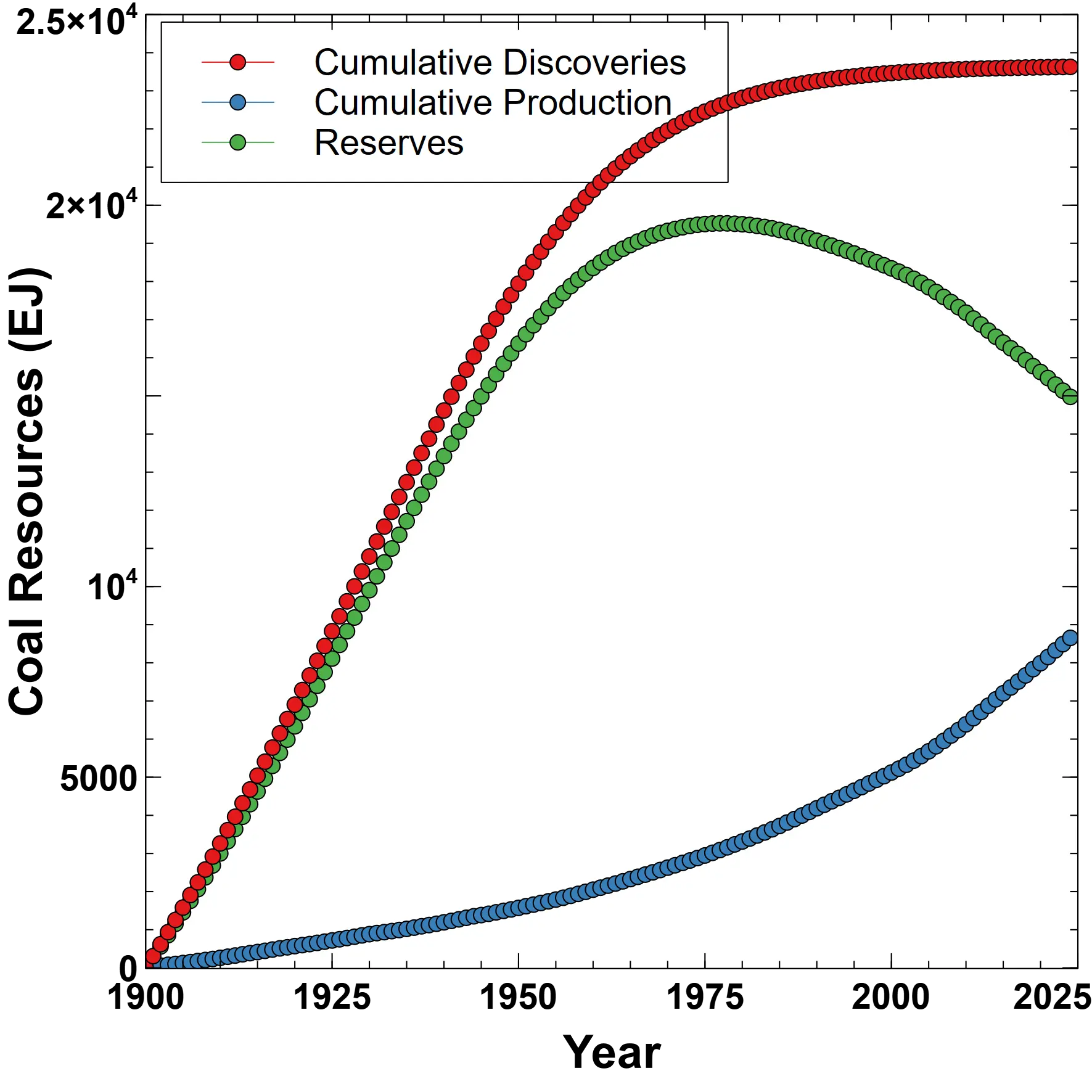
Estimated coal discoveries, production and reserves.
Coal reserves exceed total consumption to date, and provide at least a century of continued production at current rates.
Conclusions
For both oil and gas, remaining reserves are less than cumulative production to date [38]. Oil is considered the “master resource” since every aspect of modern society depends on petroleum including mining, production and transport. Oil consumption during the last 30 years is equal to all consumption prior to that time, and continues to increase in accordance with Odum’s Maximum Power Principle, while discoveries peaked in the 1960s. Our analysis shows that remaining reserves will soon become severely constrained which is in agreement with the International Energy Agency (IEA), as reported in Reuters:
The decline in output from mature global oil and gas fields is accelerating amid greater reliance on shale and deep offshore resources, the International Energy Agency said on Tuesday, meaning companies need to invest more just to keep output flat.
IEA Executive Director Fatih Birol said in an IEA statement, “Decline rates are the elephant in the room for any discussion of investment needs in oil and gas, and our new analysis shows that they have accelerated in recent years.”
As we have previously argued, there are no viable alternatives to fossil fuels for maintaining the levels of energy consumption currently enjoyed by modern society, there is no evidence that a transition to alternate energy sources will be made, and any attempt will only exacerbate the human condition of ecological overshoot. Given the physical limits of the quantities of remaining fossil fuels, it would be wise to consider society in a post-energy world.
Future Directions
This analysis highlights both the strengths and the gaps in our current understanding of global fossil fuel reserves. While backdated discoveries provide a more geologically grounded measure of what was found and when, data incompleteness and inconsistent reporting remain significant obstacles. Several directions for future research could improve both the accuracy and the policy relevance of these estimates:
- Improved Data Completeness and Transparency
- Global discovery datasets such as GOGET remain sparse, particularly for pre-1970 discoveries and small fields. Expanded access to proprietary datasets (e.g., IHS, Rystad, Wood Mackenzie) or systematic reconciliation between open and proprietary sources could substantially reduce uncertainty [6].
- Standardization of reserve reporting (proved, probable, possible) across jurisdictions would allow more consistent backdating and cross-comparison.
- Integration of Reserve Growth Dynamics
- Reserve growth from improved recovery methods and re-appraisal of fields remains one of the largest uncertainties [2,28]. Future work could integrate dynamic reserve growth functions calibrated regionally rather than assuming global averages.
- Probabilistic and Scenario-Based Models
- Deterministic logistic fits provide useful baselines, but probabilistic ensemble methods (e.g., Bayesian hierarchical models, Monte Carlo ensembles) could better capture uncertainty in discovery timing, reserve growth, and coverage fractions.
- Energy–Economy Feedbacks
- The Odum–Garrett framework implies that energy availability and economic growth are tightly coupled. Future work could explicitly link discovery-based reserve estimates to macroeconomic scenarios, testing the limits of economic growth under constrained fossil supply.
- Automation and Reproducibility
- The imputation and fitting pipeline described here is modular and extensible. Future improvements could include automated validation dashboards, uncertainty quantification tools, and direct integration with live statistical reviews (EI, IEA, EIA) for year-on-year updates.
In summary, future research must extend beyond refining the size of fossil reserves to considering their functional availability in a deindustrializing world. Better alignment of geologic, economic, and climate perspectives will be essential to assess how the remaining fossil fuels support a rapidly diminishing industrial society.
Acknowledgments
This analysis of oil, gas and coal reserves was done at the request of Simon Michaux, developer of the Venus Project: The Venus Project fosters the convergence of design and evolution to develop transition strategies in response to overshoot. The results were presented during an interview with Arnes Biogradlija of Energy News, Beyond the Green Transition: Simon Michaux’s Case for a Resource-Balanced Energy Future.
Special thanks also to Jonathan Frost for reading the initial draft, his thoughtful insights and helpful suggestions.
Related articles:
- Hubbert Linearization – An Esoteric Concept with Extraordinary Consequences
- Burning Man – The Failure of the Green New Deal
- Stefan-Boltzmann Revisited – Limits to Growth with Physics
- The Decline and Fall of the Petroleum Empire – An EROI analysis of renewable energy
- The Growing Gap – The End of an Era
References and further reading
[1] 5.5.1: Field and Well Performance of Gas Reservoirs by Material Balance | PNG 301: Introduction to Petroleum and Natural Gas Engineering. Accessed: July 29, 2025.
[2] H. B. Abdulkhaleq, K. A. Khalil, W. J. Al-Mudhafar, and D. A. Wood, Advanced machine learning for missing petrophysical property imputation applied to improve the characterization of carbonate reservoirs, Geoenergy Science and Engineering, vol. 238, p. 212900, July 2024, doi: 10.1016/j.geoen.2024.212900.
[3] S. Report, An Offshore Timeline, Coastal Review. Accessed: July 29, 2025.
[4] Approximate conversion factors. BP Statistical Review of World Energy – updated July 2021.
[5] S. Coutry, M. Tantawy, and S. Fadel, Assessing the accuracy of empirical decline curve techniques for forecasting production in unconventional reservoirs: a case study of Haynesville, Marcellus, and Marcellus Upper Shale, Journal of Engineering and Applied Science, vol. 70, no. 1, p. 69, June 2023, doi: 10.1186/s44147-023-00233-5.
[6] F. McKay, Benchmarking 2023’s upstream FIDs | Wood Mackenzie. Accessed: July 29, 2025.
[7] Coal Rank - an overview | ScienceDirect Topics. Accessed: Aug. 03, 2025.
[8] COMPARATIVE STUDY OF DECLINE CURVE ANALYSIS METHODS USING A LAB-SCALE GAS RESERVOIR - Blacklight, Accessed: July 29, 2025.
[9] Decline Analysis Curve - an overview | ScienceDirect Topics. Accessed: July 29, 2025.
[10] S. Lee, Decline Curve Analysis Essentials. Accessed: July 29, 2025.
[11] Development lead times, Edison Group. Accessed: July 29, 2025.
[12] G. Majeed, Estimation of Gas Oil Ratio, Petroleum and Coal, vol. 58, no. 01, pp. 539–550, 2016.
[13] Final Investment Decision: Meaning, Definition, and Complete Guide, Latest Global Construction Industry Projects (2024) - Blackridge Research & Consulting. Accessed: July 29, 2025.
[14] Global recoverable oil reserves hold steady at 1,536 billion barrels; insufficient to meet demand without swift electrification, Rystad Energy. Accessed: July 29, 2025.
[15] V. Smil, Halfway Between Kyoto and 2050: Zero Carbon Is a Highly Unlikely Outcome, Fraser Institute, 2024.
[16] J. Laherrère, C. A. S. Hall, and R. Bentley, How much oil remains for the world to produce? Comparing assessment methods, and separating fact from fiction, Current Research in Environmental Sustainability, vol. 4, p. 100174, 2022, doi: 10.1016/j.crsust.2022.100174.
[17] Coal Quality Workshop - Themral and Coking Coal, Accessed: Aug. 03, 2025.
[18] All Types of Coal Are Not Created Equal, Wendy Lyons Sunshine, ThoughtCo. May 13, 2025. Accessed: Aug. 03, 2025.
[19] J. W. Schmoker, T. S. Dyman, and M. Verma, Introduction to Aspects of Reserve Growth. U.S. Geological Survey Bulletin 2172–A, June 25, 2001.
[20] AONG manager, Life of an Oil or Gas Field, AONG website. Accessed: July 29, 2025.
[21] C. Xiao, G. Wang, Y. Zhang, and Y. Deng, Machine-learning-based well production prediction under geological and hydraulic fracture parameters uncertainty for unconventional shale gas reservoirs, Journal of Natural Gas Science and Engineering, vol. 106, p. 104762, Oct. 2022, doi: 10.1016/j.jngse.2022.104762.
[22] X. Tan et al., Material balance method and classification of non-uniform water invasion mode for water-bearing gas reservoirs considering the effect of water sealed gas, Natural Gas Industry B, vol. 8, no. 4, pp. 353–358, Aug. 2021, doi: 10.1016/j.ngib.2021.07.005.
[23] D. J. Stekhoven and P. Bühlmann, MissForest—non-parametric missing value imputation for mixed-type data, Bioinformatics, vol. 28, no. 1, pp. 112–118, Jan. 2012, doi: 10.1093/bioinformatics/btr597.
[24] National assessment of undiscovered conventional oil and gas resources, USGS-MMS working paper | U.S. Geological Survey. Accessed: July 29, 2025.
[25] T. R. Klett et al., New U.S. Geological Survey method for the assessment of reserve growth, U.S. Geological Survey, 2011–5163, 2011. doi: 10.3133/sir20115163.
[26] Oil and gas reserves and resource quantification, Wikipedia. June 18, 2025. Accessed: July 29, 2025.
[27] Peak Shale Amid Maximum Pessimism. Goehring & Rozencwajg Natural Resource Investors, July 2, 2025. Accessed: July 29, 2025.
[28] T. Ahmed and D. N. Meehan, Performance of Oil Reservoirs, in Advanced Reservoir Management and Engineering, Elsevier, 2012, pp. 433–483. doi: 10.1016/B978-0-12-385548-0.00004-X.
[29] Proven Reserves: What They are, How They Work, Investopedia. Accessed: July 29, 2025.
[30] T. Yehia, H. Khattab, M. Tantawy, and I. Mahgoub, Removing the Outlier from the Production Data for the Decline Curve Analysis of Shale Gas Reservoirs: A Comparative Study Using Machine Learning, ACS Omega, vol. 7, no. 36, pp. 32046–32061, Aug. 2022, doi: 10.1021/acsomega.2c03238.
[31] Reserves-to-Production Ratio: Overview, Examples, FAQ, Investopedia. Accessed: July 29, 2025.
[32] STEO Data Browser. Accessed: July 29, 2025.
[33] Cleveland, C. The history of global natural gas production, Visualizing Energy Institute for Global Sustainability - Boston University, May 20, 2024. Accessed: Aug. 03, 2025.
[34] The Life Cycle of Oil and Gas Fields. Planet Energy, August 11, 2015. Accessed: July 29, 2025.
[35] World Primary Energy Production. The Shift Project. Accessed: July 29, 2025.
[36] Clark, A. These 30 Companies Emit Nearly Half the Energy Sector’s Methane, Bloomberg, Accessed: July 29, 2025.
[37] Attanasi, E. and Coburn, T. Uncertainty and Inferred Reserve Estimates—The 1995 National Assessment. U.S. Geological Survey, Reston, Virginia: 2003. Accessed: July 29, 2025.
[38] Kuo, G. When Fossil Fuels Run Out, What Then?, The Millennium Alliance for Humanity and the Biosphere (MAHB) Stanford University, December 5, 2017. Accessed: Aug. 10, 2025.
[39] Which country has the most coal? | U.S. Geological Survey. Accessed: July 28, 2025.
[40] Gupta, A. and Hall, C. A Review of the Past and Current State of EROI Data, MDPI, October, 2011.
Image credits
- Hero: Geological Time Spiral, United States Geological Survey - Graham, Joseph, Newman, William, and Stacy, John, 2008, The geologic time spiral—A path to the past (ver. 1.1): U.S. Geological Survey General Information Product 58.
- Global Primary Energy by Source, Our World in Data.
- Discover, Production and Reserve Plots: Veusz.
Appendix - Supplementary Material and Methods
Petroleum discovery, production and reserve data is more easily obtained than gas and coal data, although not entirely transparent. Our estimates for field sizes and years of discovery come from multiple sources.
Data was obtained from the Global Energy Monitor Global Oil and Gas Extraction Tracker (GOGET), but the data is sparse. Of the 7396 oil and gas fields in the database, 2466 did not have a year of discovery and 4875 of the 42769 units did not list one or more of production, cumulative production or reserve values.
We developed a two-stage imputation pipeline to estimate missing discovery years for oil and gas fields and opening years for coal mines, utilizing data imported into a SQLite database (Energy.db). The first stage employed heuristic rules, and the second stage applied machine‐learning (specifically, Random Forest) models to residual gaps. Diagnostic checks were conducted to assess the similarity of imputed and observed data distributions. All data was normalized to a common energy unit of exajoules (EJ),
- For oil, 1 Gbl = 6.119 EJ
- For gas, 1 TCM (thousand cubic meters) = 36.0 EJ
- For coal: (1 EJ = GJ)
- Anthracite: 27.70 GJ/tonne
- Bituminous: 27.60 GJ/tonne
- Subbituminous: 18.80 GJ/tonne
- Lignite: 14.40 GJ/tonne
Data preprocessing and feature construction
We read the following tables: Oil_Gas_fields, Oil_Gas_Production_Reserves, Coal_open_mines, and Coal_closed_mines from Energy.db. Relevant predictors included production start year, FID year, status year, life-of-mine, capacity, and first observed data year. All numeric columns were coerced to numeric types, and categorical features were encoded as dummy variables. Duplicate unit records were dropped and only one record per unique Unit ID was retained.
Heuristic estimation
Missing discovery years for oil/gas were first imputed using domain-informed heuristics [3,11,13,20,34]:
- If a production start year was available, the discovery year was estimated as production year minus a median lag derived from known field data, stratified by onshore/offshore status and fuel type.
- If the FID year was available but not production year, the estimate used FID minus median lag.
- If project status text contained the word “discover” and a status year was present, we assumed discovery occurred in that year.
- Otherwise, the first data availability year was used.
For coal mines, similar heuristic logic used reported life-of-mine and status year to estimate an opening year if missing.
Machine‐learning imputation
Residual missing values (i.e. those not recovered via heuristics) were imputed using a Random Forest regressor trained on known values. Features included production year, FID year, status year, first data year, life-of-mine, and capacity. We applied mean absolute error (MAE) and root mean squared error (RMSE) evaluation during hold-out validation and retained imputations only when the model performed within acceptable error thresholds.
Random Forest–based approaches like missForest have been shown to perform well in mixed-type, non-linear imputation settings (Stekhoven & Bühlmann, 2012; Tang & Ishwaran, 2017) (arXiv) [23].
Flagging and integration
For each record, the final imputed table includes:
- The ultimate year value (
Discovery year finalorOpening year final), - The original reported year (if any),
- A discrete flag –
estimate_source– indicating whether the value was"reported", derived by heuristic logic (e.g."from_prod_year","status_year"), or predicted by Random Forest ("random_forest").
These results were written into three new SQLite tables: Oil_missing, Gas_missing, and Coal_missing, preserving provenance and enabling transparency.
Distributional diagnostics
To assess imputation plausibility, we compared the distributions of observed versus imputed values using multiple methods (Nguyen et al., 2013) (BioMed Central):
- Kernel density and box plots to visually inspect differences in distribution shape, central tendency, and spread.
- Quantile–quantile (Q–Q) plots to evaluate whether the imputed values followed the same quantile distribution as the observed data.
- Kolmogorov–Smirnov (K–S) tests, a non-parametric test for whether two samples are drawn from the same distribution, used to flag implausible divergences.
- Mann–Whitney U tests to compare median differences robustly without relying on normality assumptions.
While the K–S test is sensitive to sample size and assumptions of missingness mechanisms (“missing at random” vs “not at random”), it remains an accepted screening tool across imputation diagnostics (BioMed Central).
Validation via hold‑out experiments
For fields and mines with known discovery/opening years, we conducted hold‑out experiments: a random subset (e.g. 20 %) of known values was temporarily masked, imputation was rerun, and the imputed values were compared to their known truth. We computed MAE and RMSE to quantify imputation error and bias. These metrics guided the calibration of our Random Forest and heuristic thresholds to ensure acceptable predictive accuracy [4,5,8,9,10,30].
Software and implementation
All analyses were implemented in Python using pandas, scikit-learn (Random Forest), and missingforest as needed. Export to and from Energy.db was handled via sqlite3. Visualization and diagnostics were performed using matplotlib, seaborn, and scipy.stats. The entire pipeline is reproducible via modular functions and can be rerun or adapted to new data as required.
This methodology balances structured domain heuristics with robust machine learning imputation, all assessed using established statistical diagnostics, to produce enriched global field and mine datasets suitable for historical trend and volume analysis.
Imputing missing field data
The methods described above impute missing years or initial reserves for fields in the dataset, but the GOGET data entirely omits some smaller fields. To address this, we assumed that reserves in 1900 were small compared to later years, discoveries peaked in the 1960s and Energy Institute reserve estimates available beginning in 1980 were reasonably accurate. To estimate missing field discovery years and sizes we applied the following method [1,21,22]:
-
Align scope & inputs
- Define targets. We estimate a latent “true” discovery flow (EJ/yr) since GOGET’s observed flow is incomplete. The model used is with a time-varying coverage that rises over time because GOGET excludes small/old units (≥25 million boe reserves or ≥1 million boe/yr), so is plausibly low in early years and higher recently.
- Use consistent definitions. We anchor production and proved reserves to Energy Institute (EI) definitions (oil includes condensate & NGLs; gas uses EI’s marketed definition). This prevents scope mismatch when we later reconcile to reserves.
- Backdate sizes to discovery year. Before modeling, we apply a published reserve-growth/backdating function to each GOGET field (oil & gas) so early-year discoveries include later “growth.” USGS methods and curves are the standard starting point.
-
Build the baseline series
-
Aggregate GOGET (backdated) field sizes by discovery year to get for oil and gas. For coal (where “discoveries” ≠ national proved reserves), keep a separate track and be explicit that mine-opening reserves don’t equal country-level proved reserves.
-
Compute cumulative , cumulative production from EI, and EI proved reserves (1980+). This gives the identity residual:
-
If , GOGET under-counts cumulative discoveries by at least by year .
-
Constrain the shape of true discoveries . Impose three weak, data-backed shape constraints on the latent series:
- Low before 1900 (small intercept),
- Single broad peak in the 1960s,
- Non-negative thereafter. A flexible lognormal or skew-normal pulse plus a low recent tail works well; the “peak-in-the-1960s” prior is well supported in the literature. Second “pulses” account for offshore oil and the shale boom [27].
-
Model coverage production, : Let or a monotone spline constrained to increase with . This encodes the inclusion thresholds and data completeness—low in early decades, higher recently—without overfitting.
-
Fit and jointly under accounting constraints. Estimate parameters shape of , coverage by minimizing a constrained loss over years with EI reserves (e.g., 1980–present):
subject to:
- Observation model: (penalize deviations to respect GOGET where present).
- Shape constraints: low pre-1900; 1960s peak; .
- Monotone coverage: .
- Proved vs. 2P bridge: allow a small factor s.t. . This acknowledges EI’s “proved” vs. likely 2P backdated sizes.
-
Allocate the “missing mass” by year
- After fitting, define implied missing discoveries , giving a modified discovery list that (i) honors GOGET where it exists, (ii) adds statistically justified mass where GOGET misses fields, and (iii) satisfies the reserves identity with EI.
-
Validate with creaming-curve logic. Cumulative discoveries vs. exploration effort should “cream” (fast early gains, then flatten).
-
Nuances for each fuel type:
- Oil: Backdating (USGS) matters most. Cumulative discovered URR should not exceed credible recoverable ranges.
- Gas: Align with marketed definitions from the Energy Institute, and discovery volumes should be on the same basis (avoid raw vs. marketed mismatches).
- Coal: Treat “discoveries” as reserve additions rather than mine openings. Calibrate the additions flow so that matches EI proved reserves path; don’t infer mine-level discoveries as country-level proved reserves without explicit scaling.
-
Uncertainty bands & scenarios. We produce low/central/high versions by varying (i) the 1960s peak width/height, (ii) reserve-growth multipliers (USGS low vs. mean curves), and (iii) the coverage slope . Report shaded EJ uncertainty bands on and on implied reserves.
Code and software used
The code and data are available on Github in the World Energy Review 2025 repository as the Energy ETL Toolkit.
energy_etl/
│
├── data/
│   ├── Energy.db                          # primary SQLite database
│   └── Discoveries_Production_backdated.csv
│
├── archive/
│   ├── impute_energy_db_v0.py             # earlier pipeline experiments
│   └── impute_energy_db_v1.py
│
├── Spreadsheet data/                      # raw Excel inputs (manifest + update workbooks)
├── Text files/
│   ├── Outline.txt (this document)
│   ├── column_types.txt
│   ├── Coal_column_types.txt
│   └── diagnostics.txt
├── plots/                                 # exported charts (3 items)
├── img/                                   # placeholder, currently empty
├── venv/                                  # virtualenv scaffold (empty placeholder)
│
├── run_pipeline.py                        # CLI driver (imports import_batch, expects append/build modules)
├── import_batch.py                        # rebuild SQLite DB from manifest / raw sheets
├── summarize_fossil_fuels.py              # generate fossil fuel summary tables (long/wide)
├── build_modified_discoveries.py          # construct discoveries-by-year series
├── split_oil_gas.py                       # partition mixed fields into oil vs gas
├── fix_reserves.py                        # reserves cleanup using EI benchmarks + smoothing
├── fix_reserves_v2.py                     # enhanced reserves fixer (newer iteration)
├── calibrate_imputation.py                # calibrate reserve growth / imputation parameters
├── coverage_analysis.py                   # assess data coverage and imputation mix
├── analyze_reserves.py                    # exploratory reserve analysis helpers
├── convert_coal_to_EJ.py                  # coal-specific unit conversions
├── convert_gas_oil_to_EJ.py               # oil & gas unit conversions
├── support scripts:
│   ├── statistical_tests.py               # KS/AD/Wasserstein diagnostics on imputed data
│   ├── diagnose_missing_quantities.py     # spot missing production/discovery values
│   ├── check_tables.py                    # schema/dtype checks on DB tables
│   ├── check_results.py                   # validate result sets against expectations
│   └── fix_hardcoded.py                   # replace legacy hard-coded adjustments
├── imputation scripts:
│   ├── impute_oil_gas_db.py               # primary DB-centric imputation pipeline
│   ├── impute_oil_gas_db_v1.py            # legacy variant
│   ├── impute_oil_gas_100_percent.py      # force full coverage imputation run
│   ├── impute_oil.py                      # standalone oil workflow
│   ├── impute_gas.py                      # standalone gas workflow
│   └── impute_coal.py                     # standalone coal workflow
├── statistical fitting:
│   ├── fit_Richards.py
│   ├── fit_Richards_2Pt.py
│   ├── richards_discovery_fit_gui.py
│   └── logistic_fit.py
├── helpers & utilities:
│   ├── utils.py                           # logging, DB helpers, percent_to_float, etc.
│   ├── peek_schema.py                    # inspect SQLite schema
│   ├── _peek_cols_runtime.py              # runtime column sampling
│   └── _peek_schema_cols.py               # schema column comparison
├── verification tools:
│   ├── verify_imputation.py
│   ├── verify_100_percent.py
│   ├── impute_oil.log / impute_gas.log / impute_coal.log (latest run logs)
│   ├── impute_oil_gas_db.log              # detailed DB imputation run log
│   └── results_*.txt / results_*.tsv      # fit diagnostics per fuel
│
├── fossil_fuels_summary*.csv              # generated summary exports (wide, long, fixed variants)
├── fuels_summary_reduced*.csv             # reduced summary variants
├── fossil_fuels_reconciliation.csv        # reconciliation report
├── fossil_fuels_summary_richards_v4.csv   # richards-fit derived summary
├── modified_discoveries*.csv              # discovery datasets (raw & fixed)
└── fuels_summary_reduced_richards_*.csv   # reduced tables from Richards-fit runs
Software
- Python is an interpreted, high-level and general-purpose programming language.
- DB Browser for SQLite* (DB4S) is a high quality, visual, open source tool designed for people who want to create, search, and edit SQLite or SQLCipher database files. DB4S gives a familiar spreadsheet-like interface on the database in addition to providing a full SQL query facility. It works with Windows, macOS, and most versions of Linux and Unix.
- DBeaver Community Universal Database Tool is a free, open-source database management tool for personal projects. Manage and explore SQL databases like MySQL, MariaDB, PostgreSQL, SQLite, Apache Family, and more.
- LibreOffice is a powerful and free office suite, with a clean interface and feature-rich tools help you unleash your creativity and enhance your productivity.
- Veusz is a scientific plotting and graphing program with a graphical user interface, designed to produce publication-ready 2D and 3D plots. In addition it can be used as a module in Python for plotting.
Data sources
Discovery, production, and reserve data was obtained for each energy source. Sources are often incomplete requiring imputation of missing data in some cases (see Methods).
- Oil
- Discoveries
- Laherrère, Hall, Bentley, “How much oil remains for the world to produce?”, Fig. 4.
- Wood MacKenzie (Bloomberg, Jan. 10, 2017).
- Hart, “Peak Oil - A Turning Point for Transport”, Fig. 1.
- More recent discovery data is available from multiple sources: Global Energy Monitor, Saif Energy Ltd., DieselNet.
- Global Energy Monitor - Global Oil and Gas Extraction Tracker (GOGET).
- Production
- Energy Institute, “Statistical Review of World Energy - 2025” [32,35,36].
- Laherrère, “World oil production: past & forecasts”, Fig. 3.
- Institute for Global Sustainability, Boston University. The history of global oil production.
- Reserves
- Energy Institute.
- Discoveries
- Natural Gas
- Discoveries
- Global Energy Monitor - Global Oil and Gas Extraction Tracker (GOGET).
- Production
- Institute for Global Sustainability, Boston University. Natural gas production by country, 1900-2022
- Energy Institute.
- Our World in Data. Gas consumption by region.
- Reserves
- Energy Institute.
- Discoveries
- Coal
- Discoveries
- Global Energy Monitor - Global Coal Mine Tracker.
- Production
- Institute for Global Sustainability, Boston University. Coal production by country, 1900-2022.
- Global Energy Monitor - Global Coal Mine Tracker.
- Our World in Data. Coal production.
- Energy Institute.
- Reserves
- Energy Institute.
- Our World in Data. Coal reserves, 2020.
- Discoveries
Glossary
Energy & Measurement Units
Exajoule (EJ) A unit of energy equal to joules, or about 278 terawatt-hours. Used to compare different energy sources on a common scale. One EJ could power about 30 million U.S. homes for a year.
Primary Energy Energy in its natural form before conversion—oil in the ground, coal in a mine, sunlight hitting a solar panel. Distinct from secondary energy like electricity generated at a power plant.
Terawatt-hour (TWh) A unit of energy equal to one trillion watt-hours. A typical large power plant produces about 10 TWh per year.
Barrel of Oil Equivalent (boe) A standardized unit allowing comparison of different energy sources. One barrel of oil equivalent is approximately 6,000 cubic feet of natural gas, or 0.14 (metric) tonnes of coal.
Million Tonnes Per Annum (Mtpa) A measure of annual production rate, commonly used for coal. One million tonnes equals approximately 1.1 million U.S. short tons.
Petroleum Industry Terms
1P, 2P, 3P Reserves Classification system for oil and gas reserves based on probability of recovery:
- 1P (Proved): 90% probability of extraction—the most conservative estimate
- 2P (Proved + Probable): 50% probability—the most likely amount
- 3P (Proved + Probable + Possible): 10% probability—the optimistic estimate
API Gravity American Petroleum Institute measure of oil density. Higher numbers mean lighter, less viscous oil that’s easier to refine. Light crude has an API greater than 31.1 while heavy crude has an API less than 22.3.
Associated Gas Natural gas found in the same reservoir as crude oil, dissolved in the oil or as a “gas cap” above it. Contrasts with non-associated gas found in gas-only reservoirs.
Backdating Assigning newly discovered reserves to the year the field was originally found rather than when the additional reserves were recognized. For example, if a field discovered in 1970 is found to contain more oil in 1990, backdating credits that oil to 1970.
Bubble Point Pressure The pressure at which dissolved gas begins to come out of solution from oil as bubbles. Important for predicting how oil will behave during extraction.
FID (Final Investment Decision) The point when a company commits capital to develop a discovered field. Typically occurs 3-7 years after discovery for onshore fields, 5-15 years for offshore.
Gas-Oil Ratio (GOR) The volume of natural gas produced per unit of oil, measured in standard cubic feet per stock tank barrel (scf/stb). Varies by region: Middle East ~10-20%, North Sea ~30-40%.
Hydraulic Fracturing (Fracking) Injecting high-pressure fluid into rock formations to create fractures, allowing oil and gas to flow more easily. Enabled the U.S. shale boom starting in the 2000s.
Kerogen A waxy organic material that forms when ancient organisms are buried and subjected to heat and pressure. Further heating converts kerogen into oil and gas over millions of years.
Play A group of oil or gas fields with similar geological characteristics in the same region. For example, “the Permian Basin play” which is located in West Texas and Eastern New Mexico.
Proved Reserves Oil or gas quantities that geological and engineering data demonstrate with reasonable certainty to be recoverable from known reservoirs under existing economic and operating conditions.
Reservoir Underground rock formation containing oil, gas, or both. Must have porosity (space for fluids), permeability (interconnected pathways), and an impermeable cap rock to trap the resources.
Stock Tank Barrel (stb) A standard measure of oil volume (42 gallons) at surface conditions after gas has separated out. Distinguishes from reservoir barrels measured underground at high pressure and temperature.
Technically Recoverable Oil or gas that can be extracted with current technology, regardless of whether it’s economically viable. A broader category than “economically recoverable.”
Ultimately Recoverable Resource (URR) The total amount of a resource that will ever be extracted from a field, region, or globally—including past production, current reserves, and future discoveries.
Geological & Coal Terms
Anthracite The highest rank of coal with the most carbon content (86-97%) and highest energy density (~28 GJ/tonne). Hardest and least common type.
Bituminous Coal Medium-rank coal with 45-86% carbon content and ~28 GJ/tonne energy. Most abundant type; used for electricity generation and steelmaking.
Lignite Lowest rank of coal with 25-35% carbon content and ~14 GJ/tonne energy. Soft, crumbly, high moisture content. Sometimes called “brown coal.”
Metallurgical (Coking) Coal High-quality coal used to make coke for steel production in blast furnaces. Must have specific properties to create strong, porous coke.
Sub-bituminous Coal Coal rank between lignite and bituminous, with 35-45% carbon content and ~19 GJ/tonne energy. Common in western U.S. and Indonesia.
Statistical & Modeling Terms
Gompertz Function A mathematical curve describing growth that slows over time, often used to model mortality or resource depletion. Named after actuary Benjamin Gompertz.
Hubbert Curve (Logistic Derivative) A bell-shaped curve describing oil production over time: slow initial growth, rapid peak, then symmetric decline. Predicted U.S. peak oil in 1970.
Imputation Statistical technique for filling in missing data values based on patterns in observed data. Essential when datasets have gaps.
Kolmogorov-Smirnov Test Statistical test determining whether two datasets come from the same distribution. Used to verify that imputed values match the pattern of observed values.
Maximum Likelihood Estimation Statistical method finding parameter values that make observed data most probable. Used to determine the “best fit” for models.
Monte Carlo Method Using repeated random sampling to obtain numerical results. Named after Monaco’s Monte Carlo casino due to its use of randomness.
Poisson Distribution Probability distribution describing the number of events occurring in a fixed time interval when events happen independently at a constant average rate.
Random Forest Machine learning technique using multiple decision trees to make predictions. Like getting opinions from many experts and taking the consensus.
Richards Function (Generalized Logistic) A flexible S-shaped growth curve with an extra parameter (ν) allowing asymmetric growth. Reduces to standard logistic curve when ν=1.
Economic & Policy Terms
Maximum Power Principle Ecologist Howard Odum’s theory that systems evolving in competition maximize their rate of energy use, not efficiency. Suggests continuous growth in energy consumption is natural for economies.
Reserve-to-Production Ratio (R/P) Years of reserves remaining at current production rates. A ratio of 50 means reserves would last 50 years if production stays constant. Misleading if production is changing.
Stranded Assets Resources that lose economic value before being fully extracted, often due to climate policy or technology changes. Major concern for fossil fuel reserves.
Substitution Method Technique for comparing energy sources by adjusting non-fossil electricity to account for fossil fuel thermal inefficiencies. Multiplies renewables by 2.5× to create comparable units, though this is controversial.
Data & Research Terms
Creaming Curve Graph showing cumulative oil discovered versus exploration effort. Typically shows rapid early discoveries (“cream”) followed by flattening as best prospects are exhausted.
GOGET (Global Oil and Gas Extraction Tracker) Database maintained by Global Energy Monitor tracking oil and gas fields worldwide, including production, reserves, and ownership.
Heuristic A practical problem-solving approach using rules of thumb rather than exhaustive calculation. “Production starts 7 years after discovery” is a heuristic.
Hold-out Validation Testing a model by temporarily hiding known data, making predictions, then comparing predictions to truth. Reveals how accurate the model is.
Material Balance Accounting method tracking all inputs and outputs of a system. For oil fields: initial oil = produced oil + remaining oil + unrecovered oil.
Reserve Growth Increase in estimated recoverable resources from a field over time as technology improves and more is learned about the geology. Can be 50-100% of initial estimates.